2 Contrasts coding
2.1 Introduction
The majority of experimental works in psychology examine the difference in behavior that arises in response to exposition to experimental conditions. Whenever an experimental factor compromises more than two levels, F-statistics provide little information about the source of an effect or interaction involving this factor.
Consider an example where you measured how long people look at a different element of the picture. You presented a set of 30 pictures of natural landscapes and 30 pictures of urban scenes to 30 participants, when their eye movements were recorded. Each picture was split into face, body, and background region of interest (ROIs). You asked participants to memories those pictures for a later discrimination task.
2.1.1 Task 1.
Upload the data and using the ANOVA test examine which ROI extended an average fixation duration for a longer time and whether this effect is qualified by image type.
| subject | imageType | stimulus | imageROI | file | fixation.duration |
|---|---|---|---|---|---|
| 1 | urban | 1 | face | 1.jpg | 3.838508 |
| 1 | urban | 1 | body | 1.jpg | 5.480666 |
| 1 | urban | 1 | rImage | 1.jpg | 13.327769 |
| 1 | natural | 2 | face | 2.jpg | 16.701815 |
| 1 | natural | 2 | body | 2.jpg | 102.907577 |
| 1 | natural | 2 | rImage | 2.jpg | 6.022491 |
| 1 | urban | 3 | face | 3.jpg | 1.672553 |
| 1 | urban | 3 | body | 3.jpg | 8.513432 |
| 1 | urban | 3 | rImage | 3.jpg | 11.598428 |
| 1 | natural | 4 | face | 4.jpg | 1.364883 |
library(tidyverse)
library(lme4)
library(afex)

subj_means_aov <- df_simu %>%
  group_by(subject, imageType, imageROI) %>%
  summarise(mean_fixation.duration = mean(fixation.duration)) %>%
  ungroup()

aovLiking <- aov_4(mean_fixation.duration ~ imageType*imageROI + Error(imageType*imageROI|subject),data = subj_means_aov)

nice(aovLiking, es = "pes", sig_symbols = rep("", 4))| Effect | df | MSE | F | pes | p.value |
|---|---|---|---|---|---|
| imageType | 1, 29 | 33.57 | 30.19 | .510 | <.001 |
| imageROI | 1.85, 53.59 | 43.36 | 7.02 | .195 | .002 |
| imageType:imageROI | 1.55, 44.88 | 28.27 | 22.67 | .439 | <.001 |
ANOVA results revealed the main effect of ROI on mean fixation duration. However, it is unclear which ROIs differ from each other and how they differ. One potential strategy is to follow up on these results using t-tests. The t-test approach does not consider all the data in each test and therefore loses statistical power. It also does not generalize well to more complex models (e.g., linear mixed-effects models; LMM) and is subject to problems of multiple comparisons.
However, scientists typically have a priori expectations about the expected pattern of means. That is, we usually have specific expectations about which groups differ from each other. In our example, we would expect that longer fixations are made to the faces, than to the body, and background.
\[\begin{equation} H_{1} : \hat{\mu}_{face} > \hat{\mu}_{body} > \hat{\mu}_{background} \end{equation}\]
Given that we have a specific hypothesis about the difference, we could test specific hypotheses directly in a regression model or LMMs, which gives much more control over the analysis. In this class, we show how planned comparisons between specific conditions (groups) or clusters of conditions, are implemented as contrasts.
2.2 Types of Contrasts
Implementing planned comparison is an effective way to align expectations with the statistical model (Schad et al., 2020). We apply a set of contrasts to model differences between categories/groups/cells/conditions. In other words, we specify a priori which groups are compared to which baselines or groups. Your set of contrasts always depends on your hypothesis about the expected pattern of means.
If you do not implement planned comparisons, R will pick a default specification on its own. Remember that your hypothesis should be formally “tested instead of, rather than as a supplement to, the ordinary “omnibus” F test.” (Hays, 1973, p. 601).
There are several ways to specify contrasts. Here we consider treatment contrasts, sum contrasts, repeated contrasts, and polynomial contrasts. For the purpose of this class, we will omit the Helmert contrasts.
2.2.1 Treatment contrasts
Treatment contrast is often used in intervention studies, where one or several intervention groups receive some treatment, which are compared to a control group. For example, two treatment groups may obtain (a) psychotherapy and (b) pharmacotherapy, and they may be compared to (c) a control group of patients waiting for treatment.
In this setting, one factor has three levels. For this factor, we make two comparisons, that would reflect two hypothesis:
\[\begin{equation} H_{1} : \mu_{psychotherapy} > \mu_{control} \end{equation}\]
\[\begin{equation} H_{2} : \mu_{pharmacotherapy} > \mu_{control} \end{equation}\]
The first contrast would compare the psychotherapy group with the control group. The second contrast would compare the pharmacotherapy group with the control group.
2.2.2 Sum contrasts
Sum contrast compares each tested group not against a baseline/control condition, but instead to the average response across all groups. Consider our working example, where we compare fixation duration made to the faces, body, and background ROIs. The question of interest may be whether fixations made to the faces and body ROIs attract longer fixations than the average fixation duration across all three ROIs. This could be done with sum contrast:
\[\begin{equation} H_{1} : \hat{\mu}_{face} > \overline{\mu} \end{equation}\]
\[\begin{equation} H_{2} : \hat{\mu}_{body} > \overline{\mu} \end{equation}\]
The first contrast would compare the fixation duration made to the faces with the average fixation duration. The second contrast would compare the fixation duration made to the body with the average fixation duration.
Sum contrast also has an important role in factors with two levels, where they simply test the difference between those two-factor levels (e.g., the difference between images of natural versus urban scenes).
2.2.3 Repeated contrasts
Repeated contrasts successively test neighboring factor levels against each other. For example, in seminar 1 we were interested whether the image in the full-spectrum condition is preferred more than in a high-spatial frequency condition and whether the image in a high-spatial frequency condition is preferred more than in the low-spatial frequency condition. Repeated contrast, test exactly these differences between neighboring factor levels.
\[\begin{equation} H_{1} : \hat{\mu}_{FS} > \hat{\mu}_{HSF} > \hat{\mu}_{LSF} \end{equation}\]
2.2.4 Polynomial contrasts
Polynomial contrasts are useful when trends are of interest. Let's say that fixation duration increases with the increasing size of the ROI. That is, one may expect that fixations decrease from background to body by the same magnitude as from the body to face. In other words, we could expect here a linear trend. What is also possible with the polynomial contrasts is to test for a quadratic trend of ROI. For example, the effect between body and background ROI could be larger or smaller compared to the effect between body and face ROI.
2.3 Basic concept
Let's try to consider the simplest case. We want to compare whether image type modulates mean fixation duration.
2.3.1 Task 2.
First, calculate descriptive statistics for each condition. Second, apply lmer function to estimate the effect of image Type on a fixation duration, using the intercept-only model.
tapply(df_simu$fixation.duration, list(df_simu$imageType), mean)

lmer1a <-lmer(fixation.duration ~ imageType + (1| subject) +(1| stimulus), df_simu)

summary(lmer1a)
## urban natural
## 20.45048 25.19636
## Linear mixed model fit by REML. t-tests use Satterthwaite's method [
## lmerModLmerTest]
## Formula: fixation.duration ~ imageType + (1 | subject) + (1 | stimulus)
## Data: df_simu
##
## REML criterion at convergence: 47853
##
## Scaled residuals:
## Min 1Q Median 3Q Max
## -2.9343 -0.6085 -0.1723 0.3970 6.1440
##
## Random effects:
## Groups Name Variance Std.Dev.
## stimulus (Intercept) 49.16 7.011
## subject (Intercept) 194.35 13.941
## Residual 392.70 19.817
## Number of obs: 5400, groups: stimulus, 60; subject, 30
##
## Fixed effects:
## Estimate Std. Error df t value Pr(>|t|)
## (Intercept) 20.450 2.874 44.480 7.115 7.33e-09 ***
## imageType2 4.746 1.889 58.000 2.512 0.0148 *
## ---
## Signif. codes: 0 '***' 0.001 '**' 0.01 '*' 0.05 '.' 0.1 ' ' 1
##
## Correlation of Fixed Effects:
## (Intr)
## imageType2 -0.329What did you notice when you compare the means for each condition with the coefficients (Estimates)?
2.3.2 Task 3.
The intercept (20.450) is the mean for urban condition
The slope (imageType2: 4.746) is the difference between means for the urban and natural condition
We can summarize this information as follows:
\[\begin{equation} Intercept = \hat{\mu}_{1} \end{equation}\]
\[\begin{equation} Slope = \hat{\mu}_{2} - \hat{\mu}_{1} \end{equation}\]
2.4 Treatment contrasts - example.
How did we arrive at these particular values for the intercept and slope?
That is, why does the intercept assess the mean of urban condition F1 and how do we know the slope measures the difference in means between natural and urban?
In our model, R uses a default contrast coding of the fixed factor. R assigns TREATMENT CONTRASTS to factors. The first factor level (here: urban) is coded as 0 and the second level (here: natural) is coded as 1. You can check this when inspecting the current contrast attribute of the factor using the contrasts command:
contrasts(df_simu$imageType)## 2
## urban 0
## natural 1In R, factor levels are usually ordered alphabetically and by default, the first level is used as the baseline in TREATMENT CONTRASTS. Obviously, this default mapping will only be correct for a given data set if the levels’ alphabetical ordering matches the desired contrast coding. When it does not, it is possible to reorder the levels:
df_simu$imageType <- factor(df_simu$imageType,
                            levels = c("natural", "urban"))
contrasts(df_simu$imageType)
## urban
## natural 0
## urban 1Let's now run our model again. Look closely at the intercept value.
lmer1 <-lmer(fixation.duration ~ imageType + (1| subject) +(1| stimulus), df_simu)
summary(lmer1)
tapply(df_simu$fixation.duration, list(df_simu$imageType), mean)
## Linear mixed model fit by REML. t-tests use Satterthwaite's method [
## lmerModLmerTest]
## Formula: fixation.duration ~ imageType + (1 | subject) + (1 | stimulus)
## Data: df_simu
##
## REML criterion at convergence: 47853
##
## Scaled residuals:
## Min 1Q Median 3Q Max
## -2.9343 -0.6085 -0.1723 0.3970 6.1440
##
## Random effects:
## Groups Name Variance Std.Dev.
## stimulus (Intercept) 49.16 7.011
## subject (Intercept) 194.35 13.941
## Residual 392.70 19.817
## Number of obs: 5400, groups: stimulus, 60; subject, 30
##
## Fixed effects:
## Estimate Std. Error df t value Pr(>|t|)
## (Intercept) 25.196 2.874 44.480 8.766 3.01e-11 ***
## imageTypeurban -4.746 1.889 58.000 -2.512 0.0148 *
## ---
## Signif. codes: 0 '***' 0.001 '**' 0.01 '*' 0.05 '.' 0.1 ' ' 1
##
## Correlation of Fixed Effects:
## (Intr)
## imageTyprbn -0.329
## natural urban
## 25.19636 20.450482.5 Sum contrasts - example.
Sum contrasts codes one of the conditions as -1 and the other as + 1, effectively ‘centering’ the effects at the grand mean (GM, i.e., the mean of the two group means).
Here, we re-scale the contrast to values of -.5 and +.5 which makes the estimated slope the same as for treatment coding and easier to interpret.
## [1] -0.5  0.5
##         [,1]
## natural -0.5
## urban 0.5## Linear mixed model fit by REML. t-tests use Satterthwaite's method [
## lmerModLmerTest]
## Formula: fixation.duration ~ imageType + (1 | subject) + (1 | stimulus)
## Data: df_simu
##
## REML criterion at convergence: 47853
##
## Scaled residuals:
## Min 1Q Median 3Q Max
## -2.9343 -0.6085 -0.1723 0.3970 6.1440
##
## Random effects:
## Groups Name Variance Std.Dev.
## stimulus (Intercept) 49.16 7.011
## subject (Intercept) 194.35 13.941
## Residual 392.70 19.817
## Number of obs: 5400, groups: stimulus, 60; subject, 30
##
## Fixed effects:
## Estimate Std. Error df t value Pr(>|t|)
## (Intercept) 22.823 2.715 36.370 8.407 4.76e-10 ***
## imageType1 -4.746 1.889 58.000 -2.512 0.0148 *
## ---
## Signif. codes: 0 '***' 0.001 '**' 0.01 '*' 0.05 '.' 0.1 ' ' 1
##
## Correlation of Fixed Effects:
## (Intr)
## imageType1 0.0002.5.1 Task 4.
What did you notice when you compare the means for each condition with the coefficients (Estimates)?
The intercept (22.82342) is the GM
The slope (imageTypenatural: -4.74588) is the difference between means for the natural and urban condition
We can summarize this information as follows:
\[\begin{equation} Intercept = (\hat\mu_{1} + \hat\mu_{2})/2 \end{equation}\]
\[\begin{equation} Slope = \hat\mu_{2} - \hat\mu_{1} \end{equation}\]
Note. This is the case for balanced data, i.e., in data sets where there are no missing data points.
2.6 Repeated contrasts - example.
To compare fixation duration between face vs. body ROI, and body vs. background ROI we will use REPEATED CONTRASTS:
library(MASS)
(contrasts(df_simu$imageROI) <- contr.sdif(3))
## 2-1 3-2
## 1 -0.6666667 -0.3333333
## 2 0.3333333 -0.3333333
## 3 0.3333333 0.6666667The first row represents face ROI, the second row body ROI, and the last row background ROI. Now the first contrast (column) tests the difference between the second minus the first row, i.e., the fixation duration to body ROI minus fixation duration to face ROI. The second contrast (column) tests the difference between the third minus the second row, i.e., the difference in the fixation duration to background ROI minus the fixation duration body ROI.
Let's now run the model. What do those results represent?
## Linear mixed model fit by REML. t-tests use Satterthwaite's method [
## lmerModLmerTest]
## Formula: fixation.duration ~ imageROI + (1 | subject) + (1 | stimulus)
##    Data: df_simu
##
## REML criterion at convergence: 47817.4
##
## Scaled residuals:
##     Min      1Q  Median      3Q     Max
## -2.8624 -0.6142 -0.1751  0.3957  6.2305
##
## Random effects:
##  Groups   Name        Variance Std.Dev.
##  stimulus (Intercept)  54.01    7.349
##  subject  (Intercept) 194.36   13.941
##  Residual             389.66   19.740
## Number of obs: 5400, groups:  stimulus, 60; subject, 30
##
## Fixed effects:
##             Estimate Std. Error       df t value Pr(>|t|)
## (Intercept)   22.823      2.730   37.115   8.361 4.63e-10 ***
## imageROI2-1    3.974      0.658 5309.002   6.039 1.65e-09 ***
## imageROI3-2   -3.476      0.658 5309.002  -5.283 1.32e-07 ***
## ---
## Signif. codes:  0 '***' 0.001 '**' 0.01 '*' 0.05 '.' 0.1 ' ' 1
##
## Correlation of Fixed Effects:
##             (Intr) iROI2-
## imageROI2-1  0.000
## imageROI3-2  0.000 -0.500
Assuming that there are three levels to the ROI fixed factor, the LMM function will estimate three regression coefficients: one intercept and two slopes. What these regression coefficients test will depend on which contrast coding is specified.
2.7 Polynomial contrasts - example.
We discussed that for the example with three different ROI levels, it is possible to test the hypothesis of a linear (or quadratic or cubic) trend across all levels of ROI.
 ggplot(data.frame(x = c(-5, 5)), aes(x = x)) +
            stat_function(fun = function(x){x^3}, color="blue", lwd = 1) +
            stat_function(fun = function(x){4*x^2}, color="green", lwd = 1) +
            stat_function(fun = function(x){10*x}, color="black", lwd = 1) +
            annotate(geom="text", label = "Quadratic", x = -4, y = 95, size =5) +
            annotate(geom="text", label = "Cubic", x = -4, y = -90, size =5) +
            annotate(geom="text", label = "Linear", x = -4, y = -32, size =5)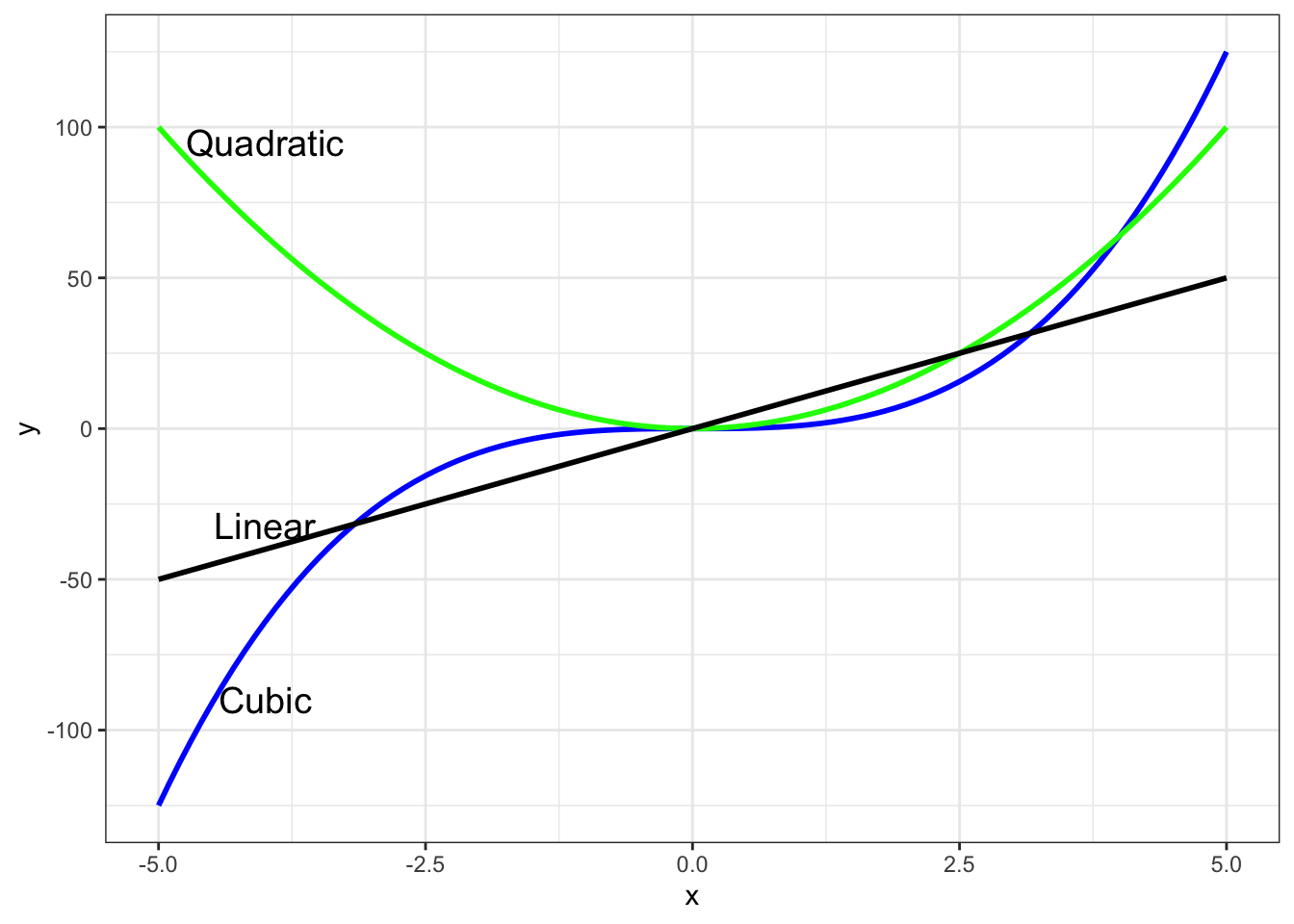
Here we assume that fixation duration increases by a constant magnitude with each successive factor level. To specify such POLYNOMIAL CONTRASTS we use the following command:
(contrasts(df_simu$imageROI) <- contr.poly(3))## .L .Q
## [1,] -7.071068e-01 0.4082483
## [2,] -7.850462e-17 -0.8164966
## [3,] 7.071068e-01 0.4082483The first column codes a linear increase with an image type. The second column codes a quadratic trend. The three rows represent three types of ROI.
Let's now run the model.
## Linear mixed model fit by REML. t-tests use Satterthwaite's method [
## lmerModLmerTest]
## Formula: fixation.duration ~ imageROI + (1 | subject) + (1 | stimulus)
##    Data: df_simu
##
## REML criterion at convergence: 47818.5
##
## Scaled residuals:
##     Min      1Q  Median      3Q     Max
## -2.8624 -0.6142 -0.1751  0.3957  6.2305
##
## Random effects:
##  Groups   Name        Variance Std.Dev.
##  stimulus (Intercept)  54.01    7.349
##  subject  (Intercept) 194.36   13.941
##  Residual             389.66   19.740
## Number of obs: 5400, groups:  stimulus, 60; subject, 30
##
## Fixed effects:
##              Estimate Std. Error        df t value Pr(>|t|)
## (Intercept)   22.8234     2.7297   37.1155   8.361 4.63e-10 ***
## imageROI.L     0.3521     0.4653 5309.0015   0.757    0.449
## imageROI.Q    -3.0414     0.4653 5309.0015  -6.537 6.87e-11 ***
## ---
## Signif. codes:  0 '***' 0.001 '**' 0.01 '*' 0.05 '.' 0.1 ' ' 1
##
## Correlation of Fixed Effects:
##            (Intr) iROI.L
## imageROI.L 0.000
## imageROI.Q 0.000  0.000
2.8 Custom contrasts
Sometimes, your hypothesis can not be expressed by a standard set of contrasts available in R. For example, a theory may make quantitative predictions about the expected pattern of means, or prior research may suggest a specific qualitative pattern. For example, let's assume that a theory may predict the pattern of mean fixation duration for each ROI which means for rImage and face are identical but the mean for the body increased linearly. We may approximate a contrast by giving a potential expected outcome of means:
\[\begin{equation} M = c(20, 20, 25) \end{equation}\]
It is possible to turn these predicted means into a contrast by centering (i.e., subtracting the mean of 21.67) them:
\[\begin{equation} M = c(-1.67, -1.67, 3.33) \end{equation}\]
We will use this contrast in a model.
df_simu$custom.imageROI <- factor(df_simu$imageROI,
                            levels = c("face", "rImage","body"))

(contrasts(df_simu$custom.imageROI) <- cbind(c(-1.67, -1.67, 3.33)))

C <- model.matrix(~1 + custom.imageROI, data = df_simu)

df_simu$custom.imageROI <- C[, "custom.imageROI1"]

lmer_custom <-lmer(fixation.duration~ custom.imageROI +
                    (1| subject) +(1| stimulus),
                  df_simu)

summary(lmer_custom )
## [,1]
## [1,] -1.67
## [2,] -1.67
## [3,] 3.33
## Linear mixed model fit by REML. t-tests use Satterthwaite's method [
## lmerModLmerTest]
## Formula: fixation.duration ~ custom.imageROI + (1 | subject) + (1 | stimulus)
## Data: df_simu
##
## REML criterion at convergence: 47822.2
##
## Scaled residuals:
## Min 1Q Median 3Q Max
## -2.8751 -0.6139 -0.1753 0.3939 6.2434
##
## Random effects:
## Groups Name Variance Std.Dev.
## stimulus (Intercept) 54.01 7.349
## subject (Intercept) 194.36 13.941
## Residual 389.63 19.739
## Number of obs: 5400, groups: stimulus, 60; subject, 30
##
## Fixed effects:
## Estimate Std. Error df t value Pr(>|t|)
## (Intercept) 22.826 2.730 37.116 8.362 4.62e-10 ***
## custom.imageROI 0.745 0.114 5310.000 6.537 6.86e-11 ***
## ---
## Signif. codes: 0 '***' 0.001 '**' 0.01 '*' 0.05 '.' 0.1 ' ' 1
##
## Correlation of Fixed Effects:
## (Intr)
## custm.mgROI 0.0002.9 Summary
TREATMENT CONTRASTS compare one or more means against a baseline condition
SUM CONTRASTS determine whether a condition’s mean is the same as the GM
REPEATED CONTRASTS compare performance between neighboring levels of a factor (e.g., high, medium, and low dosage)
POLYNOMIAL CONTRASTS tests whether there is a linear (or quadratic or cubic) trends that span across multiple factor levels.
CUSTOM CONTRASTS allows specifying a qualitative pattern of means.
2.10 What makes a good contrast?
Custom contrasts decompose ANOVA omnibus F tests into several component comparisons (Baguley, 2019).
Good contrast:
answers the research questions
is orthogonal
Orthogonality can be determined easily in R by computing the correlation between two contrasts. Orthogonal contrasts have a correlation of 0. Let's consider two factors in a 2 × 2 design using SUM CONTRASTS, these sum contrasts and their interaction are orthogonal to each other:
##      F1 F2 F1xF2
## [1,]  1  1     1
## [2,]  1 -1    -1
## [3,] -1  1    -1
## [4,] -1 -1     1
##       F1 F2 F1xF2
## F1     1  0     0
## F2     0  1     0
## F1xF2  0  0     1
2.11 Homework
Compute the model that examines the interaction between image type and ROI on mean fixation duration. Formulate a hypothesis and choose appropriate contrast that will examine your hypothesis. Report your results and include a figure that illustrates your results.
df_simu$imageType <- factor(df_simu$imageType,
                            levels = c("natural", "urban"))


df_simu$imageROI <- factor(df_simu$imageROI,
                            levels = c("body", "face", "rImage"))

str(df_simu)

df_simu$fixation.duration <- as.numeric(df_simu$fixation.duration)

lmer_task6 <-lmer(fixation.duration~ imageROI*imageType +
                    (1+imageROI*imageType| subject) +(1+imageROI*imageType| stimulus),
                  df_simu)
## Warning: Model failed to converge with 6 negative eigenvalues: -5.6e-02
## -8.3e-02 -8.8e-02 -2.3e-01 -9.7e-01 -5.2e+02
summary(lmer_task6)

# I will use effects library to show convenient (not the most elegant) way to plot predicted effects.

library(effects)
plot(allEffects(lmer_task6))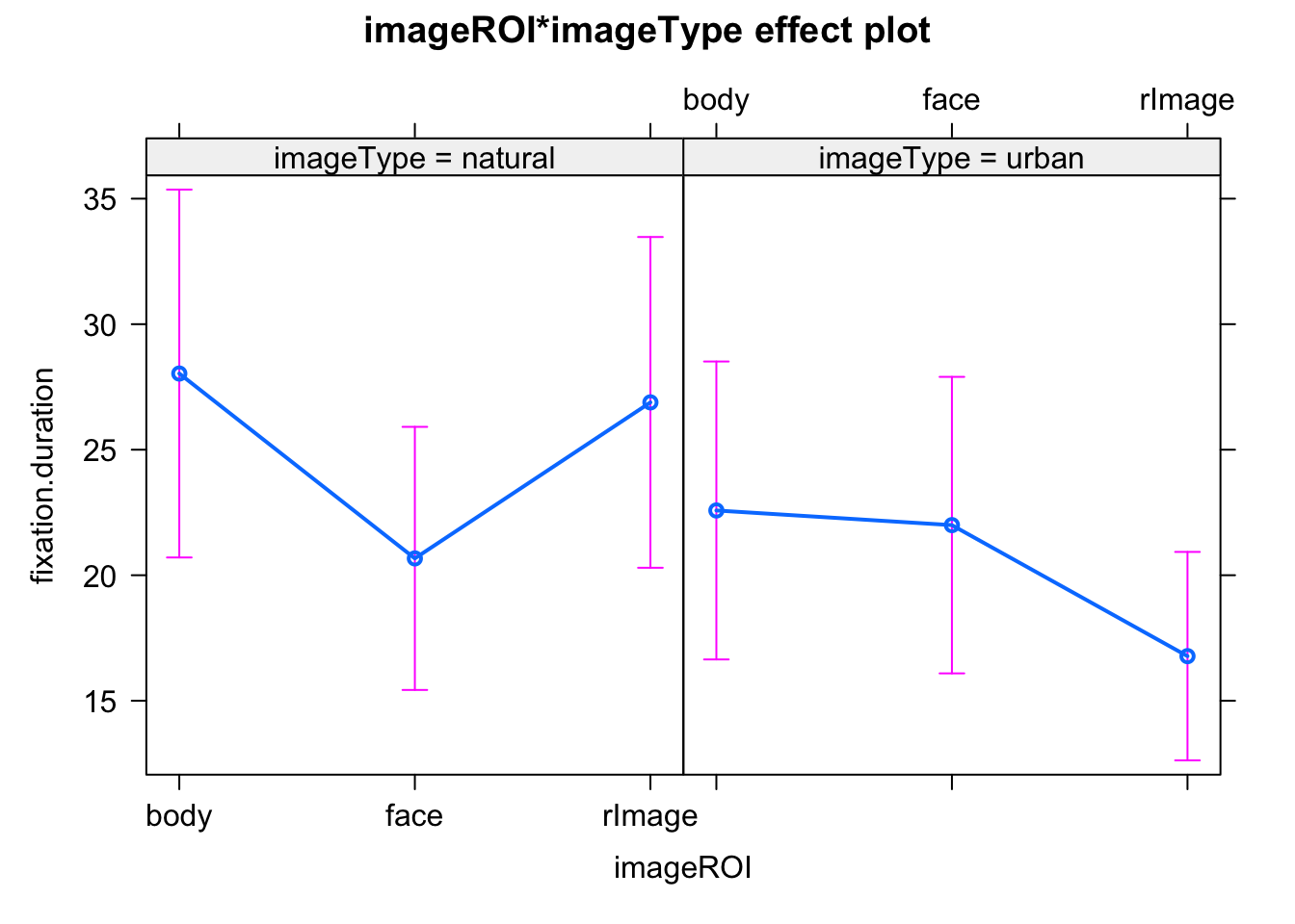
## tibble [5,400 × 7] (S3: tbl_df/tbl/data.frame)
##  $ subject          : int [1:5400] 1 1 1 1 1 1 1 1 1 1 ...
##  $ imageType        : Factor w/ 2 levels "natural","urban": 2 2 2 1 1 1 2 2 2 1 ...
##  $ stimulus         : int [1:5400] 1 1 1 2 2 2 3 3 3 4 ...
##  $ imageROI         : Factor w/ 3 levels "body","face",..: 2 1 3 2 1 3 2 1 3 2 ...
##  $ file             : chr [1:5400] "1.jpg" "1.jpg" "1.jpg" "2.jpg" ...
##  $ fixation.duration: num [1:5400] 3.84 5.48 13.33 16.7 102.91 ...
##  $ custom.imageROI  : Named num [1:5400] -1.67 3.33 -1.67 -1.67 3.33 -1.67 -1.67 3.33 -1.67 -1.67 ...
##   ..- attr(*, "names")= chr [1:5400] "1" "2" "3" "4" ...
## Linear mixed model fit by REML. t-tests use Satterthwaite's method [
## lmerModLmerTest]
## Formula:
## fixation.duration ~ imageROI * imageType + (1 + imageROI * imageType |
##     subject) + (1 + imageROI * imageType | stimulus)
##    Data: df_simu
##
## REML criterion at convergence: 47539.1
##
## Scaled residuals:
##     Min      1Q  Median      3Q     Max
## -2.8094 -0.6050 -0.1671  0.3860  6.1704
##
## Random effects:
##  Groups   Name                          Variance Std.Dev. Corr
##  stimulus (Intercept)                    72.404   8.509
##           imageROIface                    8.112   2.848   -0.99
##           imageROIrImage                 29.325   5.415   -0.51  0.60
##           imageTypeurban                 51.726   7.192   -0.52  0.51  0.37
##           imageROIface:imageTypeurban     5.685   2.384    0.63 -0.58  0.10
##           imageROIrImage:imageTypeurban  15.399   3.924   -0.01 -0.09 -0.81
##  subject  (Intercept)                   334.524  18.290
##           imageROIface                   27.674   5.261   -1.00
##           imageROIrImage                 41.655   6.454   -0.44  0.44
##           imageTypeurban                 27.928   5.285   -0.83  0.83  0.69
##           imageROIface:imageTypeurban    32.796   5.727    0.89 -0.89 -0.65
##           imageROIrImage:imageTypeurban  19.658   4.434   -0.62  0.62 -0.41
##  Residual                               365.064  19.107
##
##
##
##
##
##   0.17
##  -0.35 -0.55
##
##
##
##
##  -0.99
##   0.17 -0.28
##
## Number of obs: 5400, groups:  stimulus, 60; subject, 30
##
## Fixed effects:
##                               Estimate Std. Error     df t value Pr(>|t|)
## (Intercept)                     28.034      3.738 39.981   7.500 3.82e-09 ***
## imageROIface                    -7.364      1.416 38.899  -5.202 6.65e-06 ***
## imageROIrImage                  -1.149      1.782 39.626  -0.645 0.522864
## imageTypeurban                  -5.455      2.485 67.318  -2.196 0.031577 *
## imageROIface:imageTypeurban      6.781      1.784 47.207   3.800 0.000414 ***
## imageROIrImage:imageTypeurban   -4.654      1.897 53.555  -2.453 0.017453 *
## ---
## Signif. codes:  0 '***' 0.001 '**' 0.01 '*' 0.05 '.' 0.1 ' ' 1
##
## Correlation of Fixed Effects:
##             (Intr) imgROI imROII imgTyp iROI:T
## imageROIfac -0.834
## imagROIrImg -0.439  0.482
## imageTyprbn -0.591  0.562  0.445
## imgROIfc:mT  0.649 -0.783 -0.477 -0.574
## imgROIrIm:T -0.069 -0.087 -0.645 -0.444  0.305
## optimizer (nloptwrap) convergence code: 0 (OK)
## boundary (singular) fit: see help('isSingular')