1 Introduction to Linear (Mixed) Effects Models
1.1 Introduction
Psychologists are usually interested in measuring behavioral response that arises in response to exposition to certain types of stimulus.
Consider a simple example, where you are interested in understanding what type of visual information predicts people's preferences. You presented a set of 30 pictures of natural landscapes and 30 pictures of urban scenes to 30 participants. Each picture was presented in high-spatial frequency condition, low-spatial frequency condition, and full-spectrum condition. You asked participants about their preference response on a 5-point scale, where 1 - indicated disliked and 5 - indicated liked.
First, you are interested in testing the magnitude of the discrepancy in preference score between natural landscapes and urban scenes.
Your null hypothesis will be:
\[\begin{equation} H_{0} : \hat{\mu}_{natural} = \hat{\mu}_{urban} \end{equation}\]Your alternative hypothesis could be:
\[\begin{equation} H_{1} : \hat{\mu}_{natural} > \hat{\mu}_{urban} \end{equation}\]Import liking.csv file and use head function to get data from the first ten observations.
| subject | imageType | stimulus | imageSF | file | liking |
|---|---|---|---|---|---|
| 1 | urban | 1 | high | 1.jpg | 2 |
| 1 | urban | 1 | low | 1.jpg | 2 |
| 1 | urban | 1 | normal | 1.jpg | 3 |
| 1 | natural | 2 | high | 2.jpg | 3 |
| 1 | natural | 2 | low | 2.jpg | 5 |
| 1 | natural | 2 | normal | 2.jpg | 2 |
| 1 | urban | 3 | high | 3.jpg | 2 |
| 1 | urban | 3 | low | 3.jpg | 3 |
| 1 | urban | 3 | normal | 3.jpg | 3 |
| 1 | natural | 4 | high | 4.jpg | 2 |
We can also check the structure of the data frame using str function.
# upload some useful libraries
library(tidyverse)
library(truncnorm)
library(afex)
library(faux)

# run function
str(df_simu)
## tibble [5,400 × 6] (S3: tbl_df/tbl/data.frame)
## $ subject : int [1:5400] 1 1 1 1 1 1 1 1 1 1 ...
## $ imageType: Factor w/ 2 levels "urban","natural": 1 1 1 2 2 2 1 1 1 2 ...
## ..- attr(*, "contrasts")= num [1:2, 1] -0.5 0.5
## .. ..- attr(*, "dimnames")=List of 2
## .. .. ..$ : chr [1:2] "urban" "natural"
## .. .. ..$ : chr "2-1"
## $ stimulus : int [1:5400] 1 1 1 2 2 2 3 3 3 4 ...
## $ imageSF : Factor w/ 3 levels "high","low","normal": 1 2 3 1 2 3 1 2 3 1 ...
## ..- attr(*, "contrasts")= num [1:3, 1:2] -0.667 0.333 0.333 -0.333 -0.333 ...
## .. ..- attr(*, "dimnames")=List of 2
## .. .. ..$ : chr [1:3] "high" "low" "normal"
## .. .. ..$ : chr [1:2] "2-1" "3-2"
## $ file : chr [1:5400] "1.jpg" "1.jpg" "1.jpg" "2.jpg" ...
## $ liking : num [1:5400] 2 2 3 3 5 2 2 3 3 2 ...As you may notice the subject, stimulus, and liking score variables are not described correctly. Let's fix it!
# convert into factor variable
df_simu$subject <- as.factor(df_simu$subject)
df_simu$stimulus <- as.factor(df_simu$stimulus)

# convert into numeric variable
df_simu$liking <- as.numeric(df_simu$liking)
Now, check the structure of the data frame again.
str(df_simu)## tibble [5,400 × 6] (S3: tbl_df/tbl/data.frame)
## $ subject : Factor w/ 30 levels "1","2","3","4",..: 1 1 1 1 1 1 1 1 1 1 ...
## $ imageType: Factor w/ 2 levels "urban","natural": 1 1 1 2 2 2 1 1 1 2 ...
## ..- attr(*, "contrasts")= num [1:2, 1] -0.5 0.5
## .. ..- attr(*, "dimnames")=List of 2
## .. .. ..$ : chr [1:2] "urban" "natural"
## .. .. ..$ : chr "2-1"
## $ stimulus : Factor w/ 60 levels "1","2","3","4",..: 1 1 1 2 2 2 3 3 3 4 ...
## $ imageSF : Factor w/ 3 levels "high","low","normal": 1 2 3 1 2 3 1 2 3 1 ...
## ..- attr(*, "contrasts")= num [1:3, 1:2] -0.667 0.333 0.333 -0.333 -0.333 ...
## .. ..- attr(*, "dimnames")=List of 2
## .. .. ..$ : chr [1:3] "high" "low" "normal"
## .. .. ..$ : chr [1:2] "2-1" "3-2"
## $ file : chr [1:5400] "1.jpg" "1.jpg" "1.jpg" "2.jpg" ...
## $ liking : num [1:5400] 2 2 3 3 5 2 2 3 3 2 ...OK, looks good.
1.1.1 Task 1.
Test whether there is a difference between urban and natural scenes in the preference liking.
subj_means <- df_simu %>%
  group_by(subject, imageType) %>%
  summarise(mean_liking = mean(liking)) %>%
  ungroup()

t.test(mean_liking ~ imageType, paired = TRUE, subj_means)
##
## Paired t-test
##
## data: mean_liking by imageType
## t = -9.2222, df = 29, p-value = 4.008e-10
## alternative hypothesis: true mean difference is not equal to 0
## 95 percent confidence interval:
## -0.2801024 -0.1784161
## sample estimates:
## mean difference
## -0.2292593Using the conventional approach we computed paired sample t-test to estimate the difference between conditions. We first had to calculate means for each subject and then conduct the t-test on means, not on the raw data. Is there an alternative approach?
1.2 Linear model
We will now start working with lme4 package for R (Bates et al., 2015).
First, we need to load the lme4 package.
To calculate the effect of image type on liking response, we are going to use the lmer() function of the lme4 package. The basic syntax is
lmer(formula, data, ...)where formula expresses the structure of the underlying model in a compact format and data is the data frame where the variables mentioned in the formula can be found.
The general format of the model formula for N fixed effects (fix) and K random effects (ran) is
DV ~ fix1 + fix2 + ... + fixN + (ran1 + ran2 + ... + ranK | random_factor1)
On the left side of the bar | you put the effects you want to allow to vary over the levels of the random factor named on the right side. Usually, the right-side variable is one whose values uniquely identify individual subjects (e.g., subject).
Consider the following possible model formulas for our data and the variance-covariance matrices they construct.
| model | syntax | |
|---|---|---|
| 1 | random intercepts only | Liking ~ imageType + (1 | subject) |
| 2 | random intercepts and slopes | Liking ~ imageType + (1 + imageType | subject) |
| 3 | model 2 alternate syntax | Liking ~ imageType + (imageType | subject) |
| 4 | random slopes only | Liking ~ imageType + (0 + imageType | subject) |
| 5 | model 2 + zero-covariances | Liking ~ imageType + (imageType || subject) |
Model 1:
\[\begin{equation*} \mathbf{\sum} = \left( \begin{array}{cc} {\tau_{00}}^2 & 0 \\ 0 & 0 \\ \end{array}\right) \end{equation*}\]Models 2 and 3:
\[\begin{equation*} \mathbf{\sum} = \left( \begin{array}{cc} {\tau_{00}}^2 & \rho\tau_{00}\tau_{11} \\ \rho\tau_{00}\tau_{11} & {\tau_{11}}^2 \\ \end{array}\right) \end{equation*}\]Model 4:
\[\begin{equation*} \mathbf{\sum} = \left( \begin{array}{cc} 0 & 0 \\ 0 & {\tau_{11}}^2 \\ \end{array}\right) \end{equation*}\]Model 5:
\[\begin{equation*} \mathbf{\sum} = \left( \begin{array}{cc} {\tau_{00}}^2 & 0 \\ 0 & {\tau_{11}}^2 \\ \end{array}\right) \end{equation*}\]where:
| Parameter | Description |
|---|---|
| (_{00}) | by-subject random intercept standard deviation |
| (_{11}) | by-subject random slope standard deviation |
| () | correlation between random intercept and slope |
The most reasonable model for these data is Model 2, so we'll stick with that. Let's fit the model, storing the results in object reg.model.
## Linear mixed model fit by REML. t-tests use Satterthwaite's method [
## lmerModLmerTest]
## Formula: liking ~ imageType + (1 + imageType | subject)
## Data: df_simu
##
## REML criterion at convergence: 13011.2
##
## Scaled residuals:
## Min 1Q Median 3Q Max
## -3.5117 -0.6411 -0.0937 0.6196 3.2803
##
## Random effects:
## Groups Name Variance Std.Dev. Corr
## subject (Intercept) 0.549113 0.74102
## imageType2-1 0.004492 0.06703 0.57
## Residual 0.632124 0.79506
## Number of obs: 5400, groups: subject, 30
##
## Fixed effects:
## Estimate Std. Error df t value Pr(>|t|)
## (Intercept) 2.67981 0.13572 29.00008 19.745 < 2e-16 ***
## imageType2-1 0.22926 0.02486 29.00002 9.222 4.01e-10 ***
## ---
## Signif. codes: 0 '***' 0.001 '**' 0.01 '*' 0.05 '.' 0.1 ' ' 1
##
## Correlation of Fixed Effects:
## (Intr)
## imageTyp2-1 0.2781.2.1 Task 2.
Now compare results from the reg.model with the results from the paired t-test. What did you notice?
The conventional and regression approach gives the same t-values. The Estimate corresponds to mean difference.
1.2.2 Task 3.
OK, it's time to warm up. Let's now consider the same set of data and test to what extent preference judgment is modulated by the type of the image and spatial frequency condition.
subj_means_aov <- df_simu %>%
group_by(subject, imageType, imageSF) %>%
summarise(mean_liking = mean(liking)) %>%
ungroup()
aovLiking <- aov_4(mean_liking ~ imageType * imageSF + Error(imageType * imageSF| subject),subj_means_aov)
nice(aovLiking, es = "pes", sig_symbols = rep("", 4))
# you can also use this function:
#aov(mean_liking ~ imageType * imageSF + Error(imageType* imageSF/ subject),subj_means_aov)| Effect | df | MSE | F | pes | p.value |
|---|---|---|---|---|---|
| imageType | 1, 29 | 0.03 | 85.05 | .746 | <.001 |
| imageSF | 1.74, 50.46 | 0.06 | 10.56 | .267 | <.001 |
| imageType:imageSF | 1.83, 53.01 | 0.03 | 29.01 | .500 | <.001 |
Using the conventional approach we computed ANOVA to estimate the difference between conditions. First, we had to calculate the means for each subject and each condition and then conduct the ANOVA on means, not on the raw data.
Let's try to apply regression approach now.
reg.model2 <-lmer(liking ~ imageType*imageSF + (1+imageType*imageSF| subject), df_simu) ## Warning: Model failed to converge with 4 negative eigenvalues: -3.5e-02
## -2.4e-01 -5.1e+01 -1.5e+02
summary(reg.model2)## Linear mixed model fit by REML. t-tests use Satterthwaite's method [
## lmerModLmerTest]
## Formula: liking ~ imageType * imageSF + (1 + imageType * imageSF | subject)
## Data: df_simu
##
## REML criterion at convergence: 12842.4
##
## Scaled residuals:
## Min 1Q Median 3Q Max
## -3.6052 -0.6654 -0.0594 0.6560 3.5046
##
## Random effects:
## Groups Name Variance Std.Dev. Corr
## subject (Intercept) 0.549279 0.74113
## imageType2-1 0.001446 0.03803 1.00
## imageSF2-1 0.023082 0.15193 0.46 0.46
## imageSF3-2 0.016983 0.13032 -0.54 -0.54 0.21
## imageType2-1:imageSF2-1 0.037878 0.19462 0.34 0.34 0.71 -0.01
## imageType2-1:imageSF3-2 0.020225 0.14221 0.96 0.96 0.35 -0.43
## Residual 0.605828 0.77835
##
##
##
##
##
##
## 0.10
##
## Number of obs: 5400, groups: subject, 30
##
## Fixed effects:
## Estimate Std. Error df t value Pr(>|t|)
## (Intercept) 2.67981 0.13573 28.99863 19.744 < 2e-16 ***
## imageType2-1 0.22926 0.02229 152.24900 10.284 < 2e-16 ***
## imageSF2-1 0.13167 0.03798 27.63037 3.467 0.00174 **
## imageSF3-2 -0.18056 0.03520 28.63837 -5.129 1.83e-05 ***
## imageType2-1:imageSF2-1 0.28778 0.06289 30.83653 4.576 7.29e-05 ***
## imageType2-1:imageSF3-2 0.16556 0.05802 73.81728 2.853 0.00561 **
## ---
## Signif. codes: 0 '***' 0.001 '**' 0.01 '*' 0.05 '.' 0.1 ' ' 1
##
## Correlation of Fixed Effects:
## (Intr) imT2-1 iSF2-1 iSF3-2 iT2-1:SF2
## imageTyp2-1 0.311
## imageSF2-1 0.336 0.105
## imageSF3-2 -0.366 -0.114 -0.150
## iT2-1:SF2-1 0.194 0.060 0.291 -0.005
## iT2-1:SF3-2 0.426 0.133 0.116 -0.131 -0.345
## optimizer (nloptwrap) convergence code: 0 (OK)
## boundary (singular) fit: see help('isSingular')1.3 Conventional approach
In the example above, you would normally use a repeated measure ANOVA on the table of means calculated across participants F1 and calculated across the different items F2. It is commonly believed that if both F1 and F2 analyses revealed significant findings, then the effects will generalize to different samples of participants, assuming that participants and items in the study can each be considered random samples from larger populations (Raaijmakers et al., 1999).
This belief is not entirely true. Both, F1 and F2 analyses were developed as intermediate steps towards F' (Clark, 1973):
\[\begin{equation} F' = (MS_{T} + MS_{S × I × T}) / (MS_{T × S} + MS_{I × T}) \end{equation}\]where:
| Parameter | Description |
|---|---|
| (MS_{T}) | mean square for the treatment effect |
| (MS_{S × I × T}) | error term of the subjects by items by treatment interaction |
| (MS_{T × S}) | error term of the treatment by subjects interaction. |
| (MS_{I × T}) | error term of the items by treatment interaction. |
F′ involves the simultaneous treatment of participants and items as random factors. Unfortunately, F' cannot be computed when the data are unbalanced or when responses are missing for certain items/participants. It makes this approach difficult to be applied in practice. In contrast, the minimum bound of the F′ (F'min) proposed by Clark (1973; Coleman (1964)) can be computed quite easily from the results of separate F1 and F2 analyses:
\[\begin{equation} F'_{min}(i,j) = (F_{1} × F_{2}) / (F_{1} + F_{2}) \end{equation}\]where:
| Parameter | Description |
|---|---|
| i | represents the numerator degrees of freedom in each analysis |
| j | represents the denominator degrees of freedom |
If F′min is significant, then F′ is assumed to be significant as well (Raaijmakers et al., 1999). However, despite its initial adoption, researchers have largely abandoned F′min and have instead utilized the following criterion:
\[\begin{equation} F' = F_{1} × F_{2} \end{equation}\]The flaws associated with this approach are related to the fact that F1 ignores systematic variability due to the individual items, and F2 ignores systematic variability due to the individual subjects. As an effect, the likelihood of Type I error increases as neither is truly an appropriate description of all sources of systematic variance within the outcome e.g., response time or accuracy (Raaijmakers, 2003).
1.4 Linear Mixed-Effects Models (LMM)
1.4.1 LMM: simple model
How should we analyze such data? Recall from the example above that the lme4 formula syntax for a model with by-subject random intercepts and slopes for predictor x would be given by y ~ x + (1 + x | subject_id) where:
| Parameter | Description |
|---|---|
| y | dependent variable |
| x | fixed factor |
| 1 + x | random effects associated with fixed factor |
| participant_id | random factor for subject |
The best way to think about this bracketed part of the formula (1 + x | subject_id) is as an instruction to lme4::lmer() about how to build a covariance matrix capturing the variance introduced by the random factor of subjects. By now you should realize that this instruction would result in the estimation of a two-dimensional covariance matrix, with one dimension for intercept variance and one for slope variance:
The beauty of lmer() function is that we are not limited to the estimation of random effects for participants; we can also specify the estimation of random effects for stimuli/item by adding another term to the syntax:
y ~ x + (1 + x | subject) + (1 + x | stimulus)
Now we are estimating two independent covariance matrices, one for participants and one for stimuli/items. In the above example, both covariance matrices will have the same 2x2 structure, but this need not be the case.
1.4.2 Task 5.
Let's try to build our first model. Apply lmer function to estimate the effect of image Type on liking. Compare your results with the results of the t-test and regression model. What did you notice?
lmer1 <-lmer(liking ~ imageType + (1+imageType| subject) +(1+imageType| stimulus), df_simu) ## Warning in checkConv(attr(opt, "derivs"), opt$par, ctrl = control$checkConv, :
## Model failed to converge with max|grad| = 0.0181301 (tol = 0.002, component 1)## Linear mixed model fit by REML. t-tests use Satterthwaite's method [
## lmerModLmerTest]
## Formula: liking ~ imageType + (1 + imageType | subject) + (1 + imageType |
## stimulus)
## Data: df_simu
##
## REML criterion at convergence: 12146.2
##
## Scaled residuals:
## Min 1Q Median 3Q Max
## -3.7659 -0.6534 -0.0259 0.6141 3.3925
##
## Random effects:
## Groups Name Variance Std.Dev. Corr
## stimulus (Intercept) 0.001575 0.03968
## imageType2-1 0.451794 0.67216 -0.50
## subject (Intercept) 0.549878 0.74154
## imageType2-1 0.006980 0.08355 0.45
## Residual 0.520193 0.72124
## Number of obs: 5400, groups: stimulus, 60; subject, 30
##
## Fixed effects:
## Estimate Std. Error df t value Pr(>|t|)
## (Intercept) 2.67981 0.14260 35.09549 18.793 <2e-16 ***
## imageType2-1 0.22926 0.09085 59.93927 2.524 0.0143 *
## ---
## Signif. codes: 0 '***' 0.001 '**' 0.01 '*' 0.05 '.' 0.1 ' ' 1
##
## Correlation of Fixed Effects:
## (Intr)
## imageTyp2-1 0.038
## optimizer (nloptwrap) convergence code: 0 (OK)
## Model failed to converge with max|grad| = 0.0181301 (tol = 0.002, component 1)
##
##
##  Paired t-test
##
## data:  mean_liking by imageType
## t = -9.2222, df = 29, p-value = 4.008e-10
## alternative hypothesis: true mean difference is not equal to 0
## 95 percent confidence interval:
##  -0.2801024 -0.1784161
## sample estimates:
## mean difference
##      -0.2292593
##
## Linear mixed model fit by REML. t-tests use Satterthwaite's method [
## lmerModLmerTest]
## Formula: liking ~ imageType + (1 + imageType | subject)
##    Data: df_simu
##
## REML criterion at convergence: 13011.2
##
## Scaled residuals:
##     Min      1Q  Median      3Q     Max
## -3.5117 -0.6411 -0.0937  0.6196  3.2803
##
## Random effects:
##  Groups   Name         Variance Std.Dev. Corr
##  subject  (Intercept)  0.549113 0.74102
##           imageType2-1 0.004492 0.06703  0.57
##  Residual              0.632124 0.79506
## Number of obs: 5400, groups:  subject, 30
##
## Fixed effects:
##              Estimate Std. Error       df t value Pr(>|t|)
## (Intercept)   2.67981    0.13572 29.00008  19.745  < 2e-16 ***
## imageType2-1  0.22926    0.02486 29.00002   9.222 4.01e-10 ***
## ---
## Signif. codes:  0 '***' 0.001 '**' 0.01 '*' 0.05 '.' 0.1 ' ' 1
##
## Correlation of Fixed Effects:
##             (Intr)
## imageTyp2-1 0.2781.4.3 LMM: Advantages
- Computes F1 and F2 at the same time
- Better for unbalanced designs (e.g. due to missing values)
- Deals better with individual differences
- Smaller likelihood of Type 2 Error
1.4.4 LMM: Disadvantages
- Requires higher computational power
- Higher likelihood of Type 1 Error
- ambiguity around reporting the p-value
1.4.5 LMM: p-values
There is no need to report p-values, because a t-distribution with a high degree of freedoms approaches the z-distribution (i.e., standard-normal distribution; Baayen et al. (2008)).
|t| > 1.96
will be
p < .05
# plot z-distribution where M = 0, range: -4 to 4
curve(dnorm, -4, 4, col='black')

# add critical values
abline(v=c(-1.96,1.96), col="black", lty = 2, lwd=3)

# manipulate number of degrees of freedom to see the overlap between t-distribution and z-distribution
curve(dt(x, df=1), from=-4, to=4, col='green',add=TRUE)
curve(dt(x, df=2), from=-4, to=4, col='blue', add=TRUE)
curve(dt(x, df=30), from=-4, to=4, col='red', add=TRUE)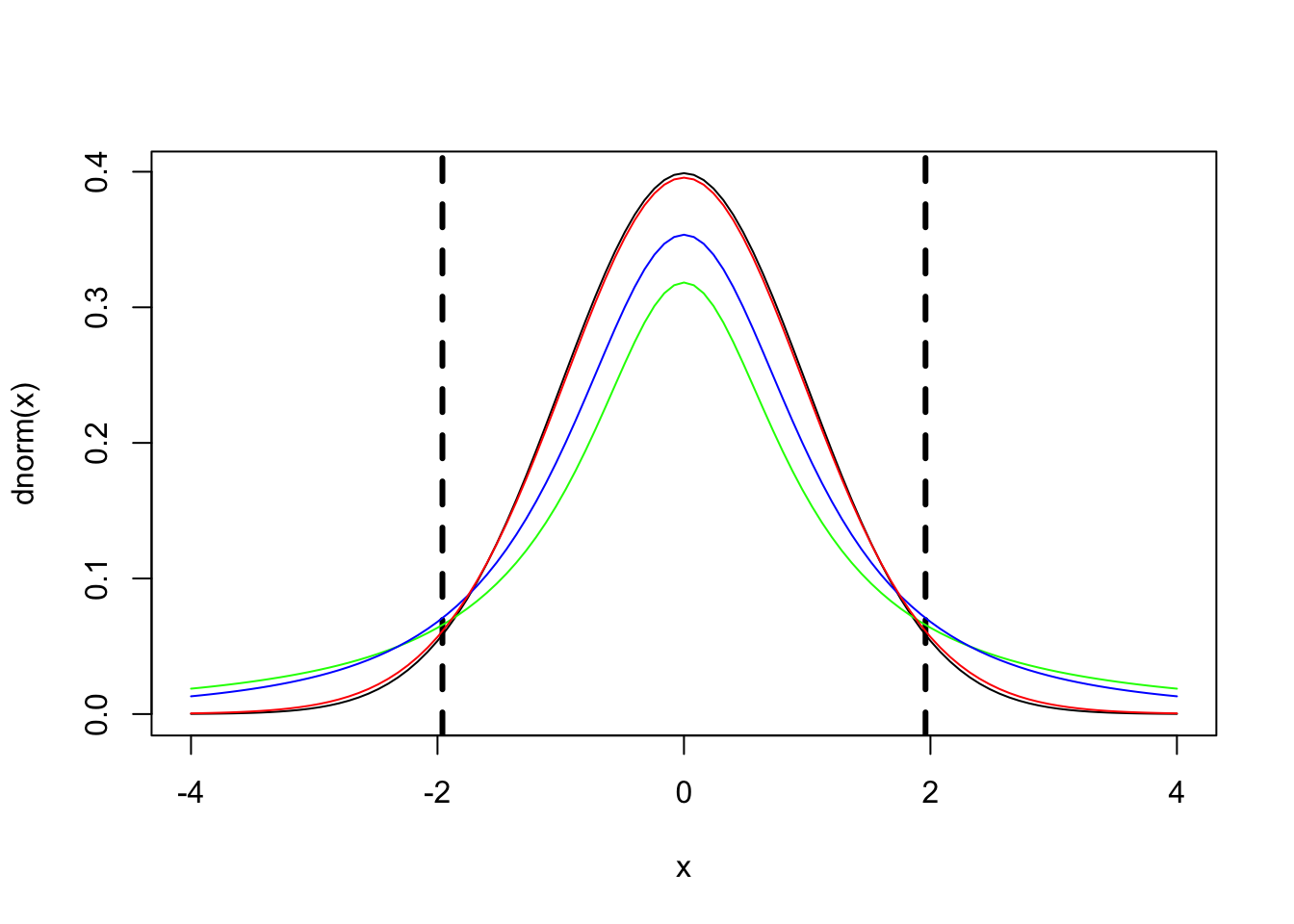
1.5 Homework
Using LME analyses, estimate the effect of image Type and spatial frequency on liking. Use the intercept-only model. Compare your results with the results of the ANOVA and regression models.
lmer_homework <-lmer(liking ~ imageSF+imageType + (1| subject) +(1| stimulus), df_simu)
summary(lmer_homework)

reg.model_homework <-lmer(liking ~ imageType+imageSF + (1+imageType+imageSF| subject), df_simu)
summary(reg.model_homework)

aov(mean_liking ~ imageType + imageSF + Error(imageType + imageSF/ subject),subj_means_aov)

aovLiking <- aov_4(mean_liking ~ imageType + imageSF + Error(imageType + imageSF| subject),subj_means_aov)

nice(aovLiking, es = "pes", sig_symbols = rep("", 4))
## Linear mixed model fit by REML. t-tests use Satterthwaite's method [
## lmerModLmerTest]
## Formula: liking ~ imageSF + imageType + (1 | subject) + (1 | stimulus)
## Data: df_simu
##
## REML criterion at convergence: 12103.7
##
## Scaled residuals:
## Min 1Q Median 3Q Max
## -3.7416 -0.6694 -0.0245 0.6335 3.4213
##
## Random effects:
## Groups Name Variance Std.Dev.
## stimulus (Intercept) 0.1145 0.3384
## subject (Intercept) 0.5498 0.7415
## Residual 0.5162 0.7185
## Number of obs: 5400, groups: stimulus, 60; subject, 30
##
## Fixed effects:
## Estimate Std. Error df t value Pr(>|t|)
## (Intercept) 2.67981 0.14258 35.11461 18.795 < 2e-16 ***
## imageSF2-1 0.13167 0.02395 5308.99996 5.498 4.02e-08 ***
## imageSF3-2 -0.18056 0.02395 5308.99996 -7.539 5.53e-14 ***
## imageType2-1 0.22926 0.08955 58.00011 2.560 0.0131 *
## ---
## Signif. codes: 0 '***' 0.001 '**' 0.01 '*' 0.05 '.' 0.1 ' ' 1
##
## Correlation of Fixed Effects:
## (Intr) iSF2-1 iSF3-2
## imageSF2-1 0.000
## imageSF3-2 0.000 -0.500
## imageTyp2-1 0.000 0.000 0.000
## Linear mixed model fit by REML. t-tests use Satterthwaite's method [
## lmerModLmerTest]
## Formula: liking ~ imageType + imageSF + (1 + imageType + imageSF | subject)
## Data: df_simu
##
## REML criterion at convergence: 12929.3
##
## Scaled residuals:
## Min 1Q Median 3Q Max
## -3.5646 -0.6377 -0.0681 0.6502 3.2987
##
## Random effects:
## Groups Name Variance Std.Dev. Corr
## subject (Intercept) 0.54918 0.7411
## imageType2-1 0.00483 0.0695 0.55
## imageSF2-1 0.02267 0.1505 0.47 0.43
## imageSF3-2 0.01648 0.1284 -0.55 0.20 0.22
## Residual 0.61703 0.7855
## Number of obs: 5400, groups: subject, 30
##
## Fixed effects:
## Estimate Std. Error df t value Pr(>|t|)
## (Intercept) 2.67981 0.13572 29.00116 19.745 < 2e-16 ***
## imageType2-1 0.22926 0.02486 29.00460 9.222 4.01e-10 ***
## imageSF2-1 0.13167 0.03796 28.99888 3.468 0.00166 **
## imageSF3-2 -0.18056 0.03514 29.00059 -5.138 1.73e-05 ***
## ---
## Signif. codes: 0 '***' 0.001 '**' 0.01 '*' 0.05 '.' 0.1 ' ' 1
##
## Correlation of Fixed Effects:
## (Intr) imT2-1 iSF2-1
## imageTyp2-1 0.278
## imageSF2-1 0.336 0.160
## imageSF3-2 -0.367 0.068 -0.149
##
## Call:
## aov(formula = mean_liking ~ imageType + imageSF + Error(imageType +
## imageSF/subject), data = subj_means_aov)
##
## Grand Mean: 2.679815
##
## Stratum 1: imageType
##
## Terms:
## imageType
## Sum of Squares 2.365191
## Deg. of Freedom 1
##
## Estimated effects are balanced
##
## Stratum 2: imageSF
##
## Terms:
## imageSF
## Sum of Squares 1.046531
## Deg. of Freedom 2
##
## Estimated effects may be unbalanced
##
## Stratum 3: imageSF:subject
##
## Terms:
## Residuals
## Sum of Squares 99.03069
## Deg. of Freedom 87
##
## Residual standard error: 1.066904
##
## Stratum 4: Within
##
## Terms:
## Residuals
## Sum of Squares 3.963142
## Deg. of Freedom 89
##
## Residual standard error: 0.2110206| Effect | df | MSE | F | pes | p.value |
|---|---|---|---|---|---|
| imageType | 1, 29 | 0.03 | 85.05 | .746 | <.001 |
| imageSF | 1.74, 50.46 | 0.06 | 10.56 | .267 | <.001 |
| imageType:imageSF | 1.83, 53.01 | 0.03 | 29.01 | .500 | <.001 |