4 Generalised Linear Mixed Effects Models
4.1 Introduction
In seminar 1, we compared conventional and multi-level modeling. In seminar 2, we learned about different types of contrasts. In seminar 3, we run the Linear Mixed Effect Models step by step. In seminar 4, we will consider non-continuous examples of dependent variables.
When psychologists are interested in the accuracy of behavioral responses they analysing a binary variable which is whether or not the participant made an error or provided a correct response. The categorical nature of the variable is often ignored. In many cases, researchers calculate the percentage of correct responses and then compute the statistical test, e.g., ANOVA. In these cases, the participant's response is treated as the continuous variable which is incorrect.
4.2 Binomial data
The Linear Mixed Effects Models (LMM) allows you to run a logistic model on binomial data. The LMM runs on the level of the single observations, and as such the variable is categorical.
The general format of the model formula for N fixed effects (fix) and K random effects (ran) is
glmer(DV ~ fix1 + ... + fixN + (ran1 + ... + ranK | random_factor1) + (ran1 + ... + ranK | random_factor2), family = binomial)
The difference between Linear Mixed Effects Models and Generalised Linear Mixed Effects Models (GLMM) is glmer command at the beginning of your model and the additional argument family = binomial that accommodates noncontinuous responses into your model.
4.3 GLMM: example
Let's consider a simple example where the intercept-only model was applied to examine to what extent participants' responses in the lexical decision task depend on word length and the participant's native language. Here we will use lexdec data file coming from library(languageR).
First, we need to add some useful packages and examine the structure of the data set.
## 'data.frame':    1659 obs. of  28 variables:
##  $ Subject       : Factor w/ 21 levels "A1","A2","A3",..: 1 1 1 1 1 1 1 1 1 1 ...
##  $ RT            : num  6.34 6.31 6.35 6.19 6.03 ...
##  $ Trial         : int  23 27 29 30 32 33 34 38 41 42 ...
##  $ Sex           : Factor w/ 2 levels "F","M": 1 1 1 1 1 1 1 1 1 1 ...
##  $ NativeLanguage: Factor w/ 2 levels "English","Other": 1 1 1 1 1 1 1 1 1 1 ...
##  $ Correct       : Factor w/ 2 levels "correct","incorrect": 1 1 1 1 1 1 1 1 1 1 ...
##  $ PrevType      : Factor w/ 2 levels "nonword","word": 2 1 1 2 1 2 2 1 1 2 ...
##  $ PrevCorrect   : Factor w/ 2 levels "correct","incorrect": 1 1 1 1 1 1 1 1 1 1 ...
##  $ Word          : Factor w/ 79 levels "almond","ant",..: 55 47 20 58 25 12 71 69 62 1 ...
##  $ Frequency     : num  4.86 4.61 5 4.73 7.67 ...
##  $ FamilySize    : num  1.386 1.099 0.693 0 3.135 ...
##  $ SynsetCount   : num  0.693 1.946 1.609 1.099 2.079 ...
##  $ Length        : int  3 4 6 4 3 10 10 8 6 6 ...
##  $ Class         : Factor w/ 2 levels "animal","plant": 1 1 2 2 1 2 2 1 2 2 ...
##  $ FreqSingular  : int  54 69 83 44 1233 26 50 63 11 24 ...
##  $ FreqPlural    : int  74 30 49 68 828 31 65 47 9 42 ...
##  $ DerivEntropy  : num  0.791 0.697 0.475 0 1.213 ...
##  $ Complex       : Factor w/ 2 levels "complex","simplex": 2 2 2 2 2 1 1 2 2 2 ...
##  $ rInfl         : num  -0.31 0.815 0.519 -0.427 0.398 ...
##  $ meanRT        : num  6.36 6.42 6.34 6.34 6.3 ...
##  $ SubjFreq      : num  3.12 2.4 3.88 4.52 6.04 3.28 5.04 2.8 3.12 3.72 ...
##  $ meanSize      : num  3.48 3 1.63 1.99 4.64 ...
##  $ meanWeight    : num  3.18 2.61 1.21 1.61 4.52 ...
##  $ BNCw          : num  12.06 5.74 5.72 2.05 74.84 ...
##  $ BNCc          : num  0 4.06 3.25 1.46 50.86 ...
##  $ BNCd          : num  6.18 2.85 12.59 7.36 241.56 ...
##  $ BNCcRatio     : num  0 0.708 0.568 0.713 0.68 ...
##  $ BNCdRatio     : num  0.512 0.497 2.202 3.591 3.228 ...
I will also remove some outliers based on the visual examination of the reaction time (RT).
densityplot(lexdec$RT)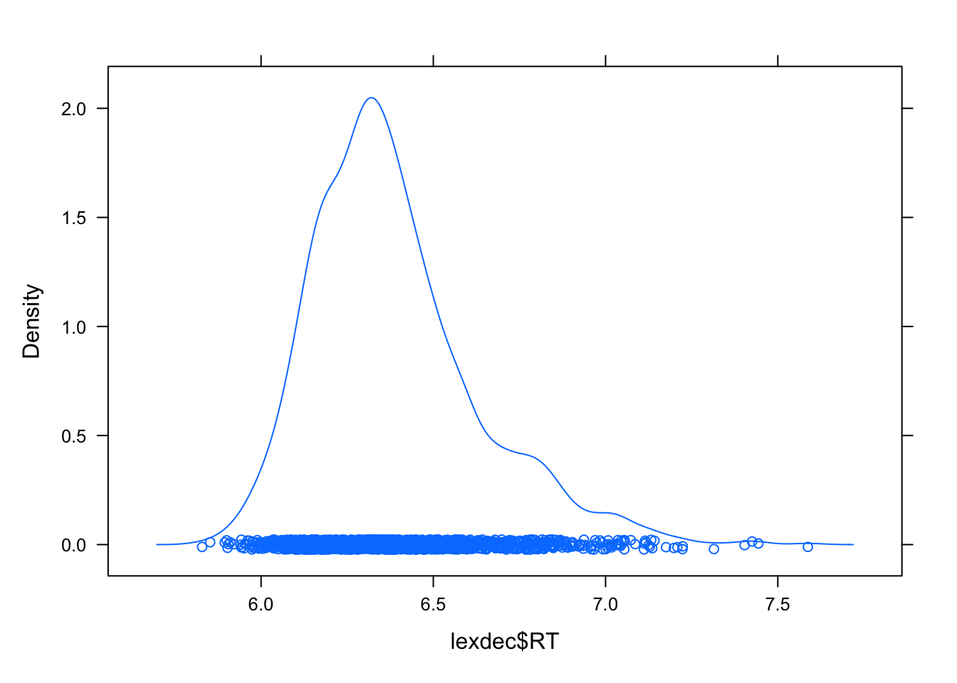
lexdec2 <- lexdec[lexdec$RT < 7 ,]
densityplot(lexdec2$RT)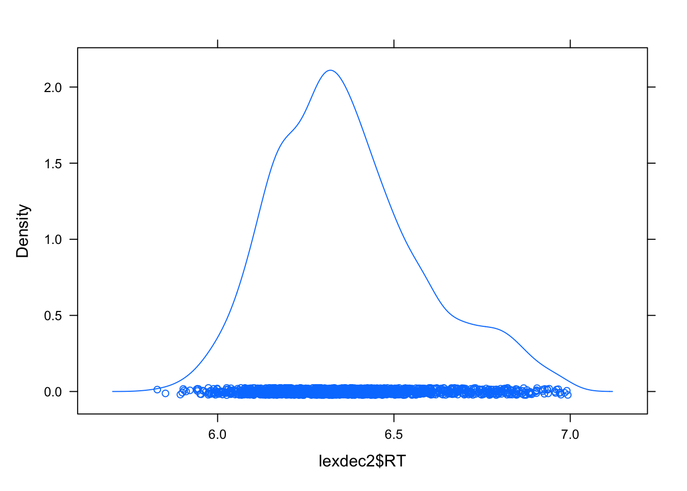
Next, we need to check if fixed and random effects are defined as factors and that your DV is in the appropriate class.
lexdec2$Subject<- as.factor(lexdec2$Subject)
lexdec2$Word <- as.factor(lexdec2$Word)
lexdec2$NativeLanguage <- as.factor(lexdec2$NativeLanguage)

# I will transform "correct" to 1 and "incorrect" to 0 and code it as a categorical variable!
lexdec2$Correct <- as.factor(ifelse(lexdec2$Correct == "correct", 1, 0))
str(lexdec2)
## 'data.frame': 1618 obs. of 28 variables:
## $ Subject : Factor w/ 21 levels "A1","A2","A3",..: 1 1 1 1 1 1 1 1 1 1 ...
## $ RT : num 6.34 6.31 6.35 6.19 6.03 ...
## $ Trial : int 23 27 29 30 32 33 34 38 41 42 ...
## $ Sex : Factor w/ 2 levels "F","M": 1 1 1 1 1 1 1 1 1 1 ...
## $ NativeLanguage: Factor w/ 2 levels "English","Other": 1 1 1 1 1 1 1 1 1 1 ...
## $ Correct : Factor w/ 2 levels "0","1": 2 2 2 2 2 2 2 2 2 2 ...
## $ PrevType : Factor w/ 2 levels "nonword","word": 2 1 1 2 1 2 2 1 1 2 ...
## $ PrevCorrect : Factor w/ 2 levels "correct","incorrect": 1 1 1 1 1 1 1 1 1 1 ...
## $ Word : Factor w/ 79 levels "almond","ant",..: 55 47 20 58 25 12 71 69 62 1 ...
## $ Frequency : num 4.86 4.61 5 4.73 7.67 ...
## $ FamilySize : num 1.386 1.099 0.693 0 3.135 ...
## $ SynsetCount : num 0.693 1.946 1.609 1.099 2.079 ...
## $ Length : int 3 4 6 4 3 10 10 8 6 6 ...
## $ Class : Factor w/ 2 levels "animal","plant": 1 1 2 2 1 2 2 1 2 2 ...
## $ FreqSingular : int 54 69 83 44 1233 26 50 63 11 24 ...
## $ FreqPlural : int 74 30 49 68 828 31 65 47 9 42 ...
## $ DerivEntropy : num 0.791 0.697 0.475 0 1.213 ...
## $ Complex : Factor w/ 2 levels "complex","simplex": 2 2 2 2 2 1 1 2 2 2 ...
## $ rInfl : num -0.31 0.815 0.519 -0.427 0.398 ...
## $ meanRT : num 6.36 6.42 6.34 6.34 6.3 ...
## $ SubjFreq : num 3.12 2.4 3.88 4.52 6.04 3.28 5.04 2.8 3.12 3.72 ...
## $ meanSize : num 3.48 3 1.63 1.99 4.64 ...
## $ meanWeight : num 3.18 2.61 1.21 1.61 4.52 ...
## $ BNCw : num 12.06 5.74 5.72 2.05 74.84 ...
## $ BNCc : num 0 4.06 3.25 1.46 50.86 ...
## $ BNCd : num 6.18 2.85 12.59 7.36 241.56 ...
## $ BNCcRatio : num 0 0.708 0.568 0.713 0.68 ...
## $ BNCdRatio : num 0.512 0.497 2.202 3.591 3.228 ...Now, we will center our continuous predictor.
lexdec2$c.Length <- lexdec2$Length - mean(lexdec2$Length) We also will establish a sum contrast to compare each tested group not against a baseline/control condition, but instead to the average response across all groups.
## [1] -0.5  0.5
##         [,1]
## English -0.5
## Other    0.5
Finally, I will run the model and plot the effects. Note, that I was specifically asked here to run an intercept-only model.
glmer_1 <-glmer(Correct ~ NativeLanguage*c.Length +
                    (1| Subject) +(1| Word),
                  lexdec2, family = binomial)
summary(glmer_1)

library(effects)
plot(allEffects(glmer_1))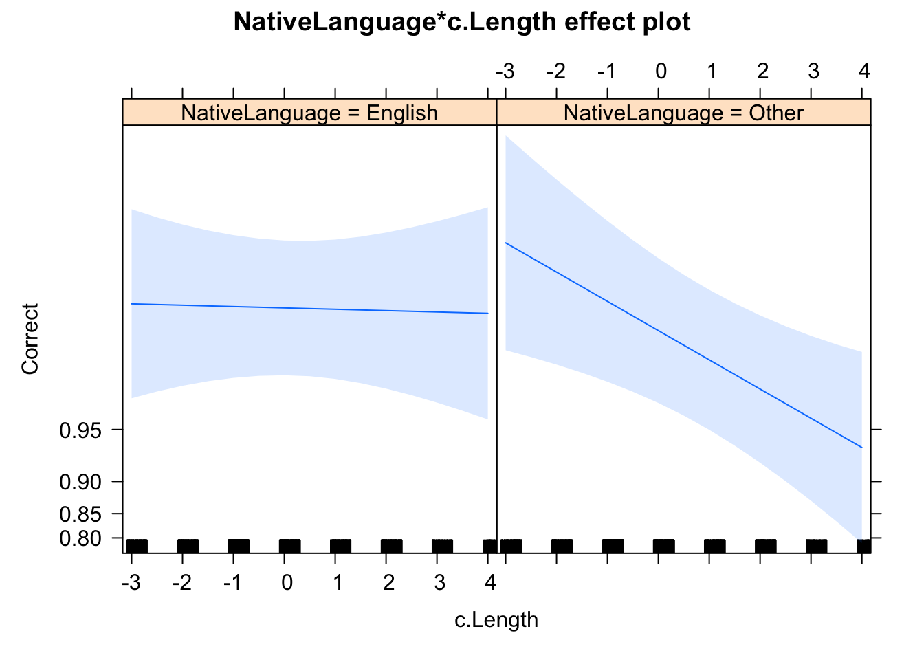
## Generalized linear mixed model fit by maximum likelihood (Laplace
##   Approximation) [glmerMod]
##  Family: binomial  ( logit )
## Formula: Correct ~ NativeLanguage * c.Length + (1 | Subject) + (1 | Word)
##    Data: lexdec2
##
##      AIC      BIC   logLik deviance df.resid
##    469.1    501.4   -228.6    457.1     1612
##
## Scaled residuals:
##     Min      1Q  Median      3Q     Max
## -9.5387  0.0702  0.1017  0.1711  0.9799
##
## Random effects:
##  Groups  Name        Variance Std.Dev.
##  Word    (Intercept) 2.2021   1.4840
##  Subject (Intercept) 0.8368   0.9148
## Number of obs: 1618, groups:  Word, 79; Subject, 21
##
## Fixed effects:
##                          Estimate Std. Error z value Pr(>|z|)
## (Intercept)                4.5308     0.4404  10.289   <2e-16 ***
## NativeLanguage1           -0.3262     0.5245  -0.622   0.5340
## c.Length                  -0.2200     0.1313  -1.675   0.0939 .
## NativeLanguage1:c.Length  -0.4008     0.1634  -2.453   0.0142 *
## ---
## Signif. codes:  0 '***' 0.001 '**' 0.01 '*' 0.05 '.' 0.1 ' ' 1
##
## Correlation of Fixed Effects:
##             (Intr) NtvLn1 c.Lngt
## NativeLngg1  0.084
## c.Length    -0.154 -0.082
## NtvLngg1:.L -0.169 -0.149 -0.013
4.4 GLMM: output
Close examination of the output tells us that t-values were replaced with z-values. Remember that the z-distribution is a standard-normal distribution that immediately tells us which of the fixed factors is significant under the following principle:
|z| > 1.96
will be
p < .05
# plot z-distribution where M = 0, range: -4 to 4
curve(dnorm, -4, 4, col='black')
# add critical values
abline(v=c(-1.96,1.96), col="black", lty = 2, lwd=3)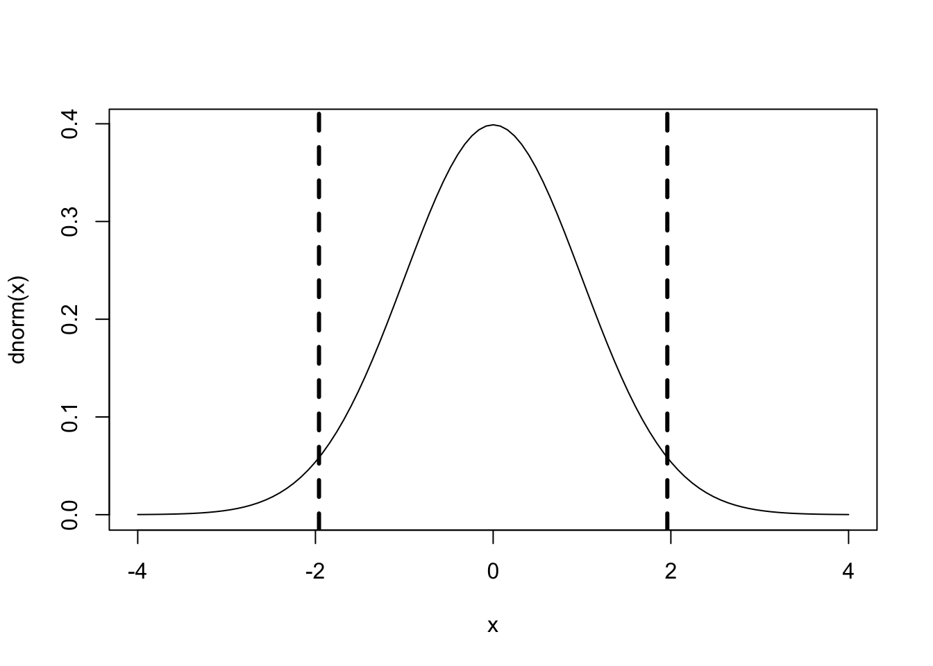 With respect to Estimates values of the fixed factors, they are not directly interpreted. They represent logit units. Given that, to calculate the predicted means for your model, first, you will need to calculate the logit values for each condition and then transform them into probabilities.
\[\begin{equation} logit = ln(\frac{p}{1-p}) \end{equation}\]
where p is a probability
We can transform this value into the probability scale:
\[\begin{equation} p = \frac{1}{1+exp(-logit)} \end{equation}\]
4.5 LMM/GLMM: Table
For the sake of transparency, we usually report the full results of your analysis in the table. For example, we will use tab_model function coming from library(sjPlot) to get a nice table of results.
summary(glmer_1)
library(sjPlot)
tab_model(glmer_1,
          show.ci = FALSE,
          show.se = TRUE,
          show.re.var = FALSE,
          show.ngroups = FALSE,
          show.icc = FALSE,
          show.obs = FALSE,
          show.r2 = FALSE, string.se = "SE",
          show.stat = TRUE, string.stat = "z-value")
## Generalized linear mixed model fit by maximum likelihood (Laplace
## Approximation) [glmerMod]
## Family: binomial ( logit )
## Formula: Correct ~ NativeLanguage * c.Length + (1 | Subject) + (1 | Word)
## Data: lexdec2
##
## AIC BIC logLik deviance df.resid
## 469.1 501.4 -228.6 457.1 1612
##
## Scaled residuals:
## Min 1Q Median 3Q Max
## -9.5387 0.0702 0.1017 0.1711 0.9799
##
## Random effects:
## Groups Name Variance Std.Dev.
## Word (Intercept) 2.2021 1.4840
## Subject (Intercept) 0.8368 0.9148
## Number of obs: 1618, groups: Word, 79; Subject, 21
##
## Fixed effects:
## Estimate Std. Error z value Pr(>|z|)
## (Intercept) 4.5308 0.4404 10.289 <2e-16 ***
## NativeLanguage1 -0.3262 0.5245 -0.622 0.5340
## c.Length -0.2200 0.1313 -1.675 0.0939 .
## NativeLanguage1:c.Length -0.4008 0.1634 -2.453 0.0142 *
## ---
## Signif. codes: 0 '***' 0.001 '**' 0.01 '*' 0.05 '.' 0.1 ' ' 1
##
## Correlation of Fixed Effects:
## (Intr) NtvLn1 c.Lngt
## NativeLngg1 0.084
## c.Length -0.154 -0.082
## NtvLngg1:.L -0.169 -0.149 -0.013| Correct | ||||
|---|---|---|---|---|
| Predictors | Odds Ratios | SE | z-value | p |
| (Intercept) | 92.83 | 40.88 | 10.29 | <0.001 |
| NativeLanguage1 | 0.72 | 0.38 | -0.62 | 0.534 |
| c Length | 0.80 | 0.11 | -1.67 | 0.094 |
|
NativeLanguage1 × c Length |
0.67 | 0.11 | -2.45 | 0.014 |
Notice that the estimates were transformed into Odds Ratios. I will use exp() to transform the estimate coefficient of the Native Language from logit units to odds ratios to demonstrate the correspondence between these scores.
exp(-0.3262)## [1] 0.7216608You may find more about the conversions of logit units to odds ratio here.
4.6 LMM/GLMM: write-up
We can summaries our results as follow:
There is no significant evidence that the effect of native language and word length did influence the accuracy of response. More importantly the interaction between native language and word length was significant. Specifically, non-native speakers were more likely to make an error response for longer words.
4.7 Task 1
Let's warm up!
Using lexdec data file test to what extent accuracy is predicted by word complexity (i.e., Complex) and whether this effect is modulated by the position of a trial in the experiment (i.e., Trial). Establish appropriate random structure. Apply Treatment contrast to test the hypothesis that simpler words are easier to process than complex ones. Create the table and write-up the results.
lexdec2$c.Trial <- lexdec2$Trial - mean(lexdec2$Trial)

lexdec2$Complex<- factor(lexdec2$Complex,
                            levels = c("simplex", "complex"))
contrasts(lexdec2$Complex)

glmer_task1 <-glmer(Correct ~ Complex*c.Trial +
                    (1| Subject) +(1| Word),
                  lexdec2, family = binomial)
summary(glmer_task1)

tab_model(glmer_task1,
          show.ci = FALSE,
          show.se = TRUE,
          show.re.var = FALSE,
          show.ngroups = FALSE,
          show.icc = FALSE,
          show.obs = FALSE,
          show.r2 = FALSE, string.se = "SE",
          show.stat = TRUE, string.stat = "z-value")
## complex
## simplex 0
## complex 1
## Generalized linear mixed model fit by maximum likelihood (Laplace
## Approximation) [glmerMod]
## Family: binomial ( logit )
## Formula: Correct ~ Complex * c.Trial + (1 | Subject) + (1 | Word)
## Data: lexdec2
##
## AIC BIC logLik deviance df.resid
## 476.4 508.8 -232.2 464.4 1612
##
## Scaled residuals:
## Min 1Q Median 3Q Max
## -8.5032 0.0692 0.1020 0.1722 1.0670
##
## Random effects:
## Groups Name Variance Std.Dev.
## Word (Intercept) 2.3143 1.5213
## Subject (Intercept) 0.8698 0.9326
## Number of obs: 1618, groups: Word, 79; Subject, 21
##
## Fixed effects:
## Estimate Std. Error z value Pr(>|z|)
## (Intercept) 4.524916 0.457495 9.891 <2e-16 ***
## Complexcomplex 0.234522 0.836932 0.280 0.7793
## c.Trial 0.001325 0.003266 0.406 0.6849
## Complexcomplex:c.Trial -0.019473 0.011794 -1.651 0.0987 .
## ---
## Signif. codes: 0 '***' 0.001 '**' 0.01 '*' 0.05 '.' 0.1 ' ' 1
##
## Correlation of Fixed Effects:
## (Intr) Cmplxc c.Tril
## Complxcmplx -0.230
## c.Trial 0.032 -0.011
## Cmplxcmp:.T -0.027 -0.453 -0.279| Correct | ||||
|---|---|---|---|---|
| Predictors | Odds Ratios | SE | z-value | p |
| (Intercept) | 92.29 | 42.22 | 9.89 | <0.001 |
| Complex [complex] | 1.26 | 1.06 | 0.28 | 0.779 |
| c Trial | 1.00 | 0.00 | 0.41 | 0.685 |
|
Complex [complex] × c Trial |
0.98 | 0.01 | -1.65 | 0.099 |
4.8 Homework
Using lexdec data file test to what extent accuracy is predicted by the interaction between word length and participants' native language. In your model control for the effect of trial and word frequency (i.e., Frequency). Conduct intercept-only model. Create the table and write-up the results.
lexdec2$c.Frequency <- lexdec2$Frequency - mean(lexdec2$Frequency)

glmer_task2 <-glmer(Correct ~ NativeLanguage*c.Length + c.Trial + c.Frequency +
                    (1| Subject) +(1| Word),
                  lexdec2, family = binomial)
summary(glmer_task2)

tab_model(glmer_task2,
          show.ci = FALSE,
          show.se = TRUE,
          show.re.var = FALSE,
          show.ngroups = FALSE,
          show.icc = FALSE,
          show.obs = FALSE,
          show.r2 = FALSE, string.se = "SE",
          show.stat = TRUE, string.stat = "z-value")
## Generalized linear mixed model fit by maximum likelihood (Laplace
## Approximation) [glmerMod]
## Family: binomial ( logit )
## Formula: Correct ~ NativeLanguage * c.Length + c.Trial + c.Frequency +
## (1 | Subject) + (1 | Word)
## Data: lexdec2
##
## AIC BIC logLik deviance df.resid
## 465.6 508.7 -224.8 449.6 1610
##
## Scaled residuals:
## Min 1Q Median 3Q Max
## -8.2263 0.0725 0.1090 0.1705 0.9602
##
## Random effects:
## Groups Name Variance Std.Dev.
## Word (Intercept) 1.5377 1.2400
## Subject (Intercept) 0.8485 0.9211
## Number of obs: 1618, groups: Word, 79; Subject, 21
##
## Fixed effects:
## Estimate Std. Error z value Pr(>|z|)
## (Intercept) 4.4457678 0.4149259 10.715 < 2e-16 ***
## NativeLanguage1 -0.3279128 0.5274023 -0.622 0.53411
## c.Length -0.0452021 0.1309964 -0.345 0.73005
## c.Trial -0.0003313 0.0030841 -0.107 0.91444
## c.Frequency 0.5460114 0.1937362 2.818 0.00483 **
## NativeLanguage1:c.Length -0.4052244 0.1643206 -2.466 0.01366 *
## ---
## Signif. codes: 0 '***' 0.001 '**' 0.01 '*' 0.05 '.' 0.1 ' ' 1
##
## Correlation of Fixed Effects:
## (Intr) NtvLn1 c.Lngt c.Tril c.Frqn
## NativeLngg1 0.090
## c.Length -0.039 -0.087
## c.Trial -0.006 0.020 -0.032
## c.Frequency 0.198 -0.007 0.417 0.001
## NtvLngg1:.L -0.172 -0.150 -0.043 -0.022 -0.052| Correct | ||||
|---|---|---|---|---|
| Predictors | Odds Ratios | SE | z-value | p |
| (Intercept) | 85.27 | 35.38 | 10.71 | <0.001 |
| NativeLanguage1 | 0.72 | 0.38 | -0.62 | 0.534 |
| c Length | 0.96 | 0.13 | -0.35 | 0.730 |
| c Trial | 1.00 | 0.00 | -0.11 | 0.914 |
| c Frequency | 1.73 | 0.33 | 2.82 | 0.005 |
|
NativeLanguage1 × c Length |
0.67 | 0.11 | -2.47 | 0.014 |