3 Linear Mixed Effect Models
3.1 Introduction
In seminar 1, we compared conventional and multi-level modeling. In seminar 2, we learned about different types of contrasts. In seminar 3, we will run a couple of Linear Mixed Effect Models from scratch.
For each analysis, you should consider (at least) eight steps:
- Import data and check the class of the variables
- Check if it is necessary to transform your data
- Remove outlines
- Identify fixed and random effects
- Center continuous predictors
- Choose appropriate contrasts
- Define the random structure
- Plot and interpret your results.
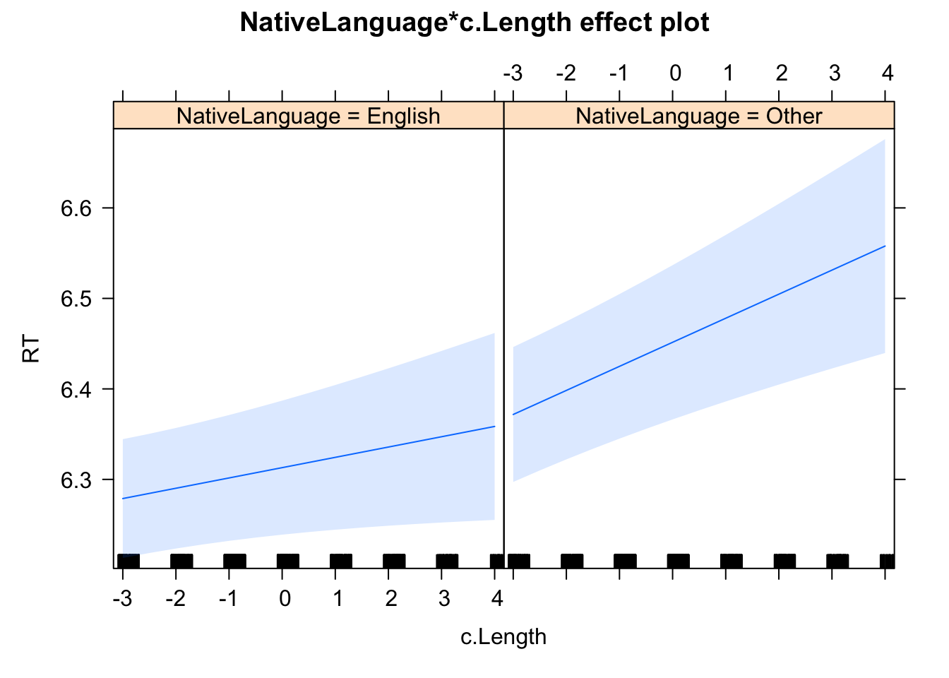
Let's go through an example. Here we will use lexdec data file coming from library(languageR). We want to examine to what extent RT depends on word length and the participant's native language.
3.2 Import data and check class of the variables
Check if your random-effects and fixed-effect factors are properly defined.
## 'data.frame':    1659 obs. of  28 variables:
##  $ Subject       : Factor w/ 21 levels "A1","A2","A3",..: 1 1 1 1 1 1 1 1 1 1 ...
##  $ RT            : num  6.34 6.31 6.35 6.19 6.03 ...
##  $ Trial         : int  23 27 29 30 32 33 34 38 41 42 ...
##  $ Sex           : Factor w/ 2 levels "F","M": 1 1 1 1 1 1 1 1 1 1 ...
##  $ NativeLanguage: Factor w/ 2 levels "English","Other": 1 1 1 1 1 1 1 1 1 1 ...
##  $ Correct       : Factor w/ 2 levels "correct","incorrect": 1 1 1 1 1 1 1 1 1 1 ...
##  $ PrevType      : Factor w/ 2 levels "nonword","word": 2 1 1 2 1 2 2 1 1 2 ...
##  $ PrevCorrect   : Factor w/ 2 levels "correct","incorrect": 1 1 1 1 1 1 1 1 1 1 ...
##  $ Word          : Factor w/ 79 levels "almond","ant",..: 55 47 20 58 25 12 71 69 62 1 ...
##  $ Frequency     : num  4.86 4.61 5 4.73 7.67 ...
##  $ FamilySize    : num  1.386 1.099 0.693 0 3.135 ...
##  $ SynsetCount   : num  0.693 1.946 1.609 1.099 2.079 ...
##  $ Length        : int  3 4 6 4 3 10 10 8 6 6 ...
##  $ Class         : Factor w/ 2 levels "animal","plant": 1 1 2 2 1 2 2 1 2 2 ...
##  $ FreqSingular  : int  54 69 83 44 1233 26 50 63 11 24 ...
##  $ FreqPlural    : int  74 30 49 68 828 31 65 47 9 42 ...
##  $ DerivEntropy  : num  0.791 0.697 0.475 0 1.213 ...
##  $ Complex       : Factor w/ 2 levels "complex","simplex": 2 2 2 2 2 1 1 2 2 2 ...
##  $ rInfl         : num  -0.31 0.815 0.519 -0.427 0.398 ...
##  $ meanRT        : num  6.36 6.42 6.34 6.34 6.3 ...
##  $ SubjFreq      : num  3.12 2.4 3.88 4.52 6.04 3.28 5.04 2.8 3.12 3.72 ...
##  $ meanSize      : num  3.48 3 1.63 1.99 4.64 ...
##  $ meanWeight    : num  3.18 2.61 1.21 1.61 4.52 ...
##  $ BNCw          : num  12.06 5.74 5.72 2.05 74.84 ...
##  $ BNCc          : num  0 4.06 3.25 1.46 50.86 ...
##  $ BNCd          : num  6.18 2.85 12.59 7.36 241.56 ...
##  $ BNCcRatio     : num  0 0.708 0.568 0.713 0.68 ...
##  $ BNCdRatio     : num  0.512 0.497 2.202 3.591 3.228 ...
3.3 Check if it is necessary to transform your data
Check if your DV is normally distributed.
Note. In this case, RT has been already log-transformed
qqnorm(lexdec$RT)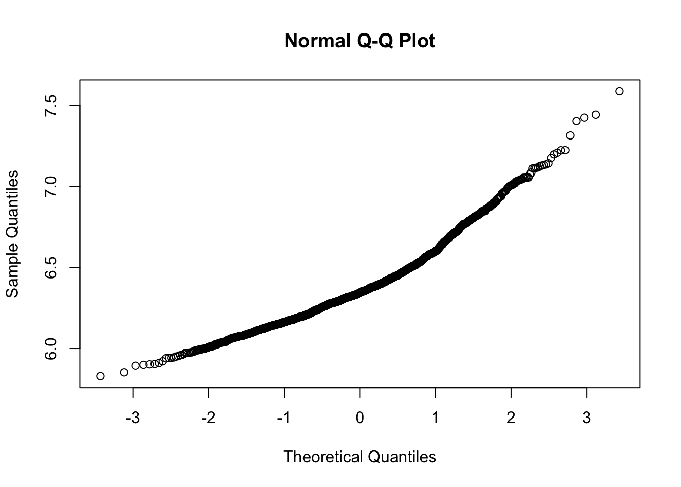
# across participants
 qqmath(~RT|Subject,data=lexdec)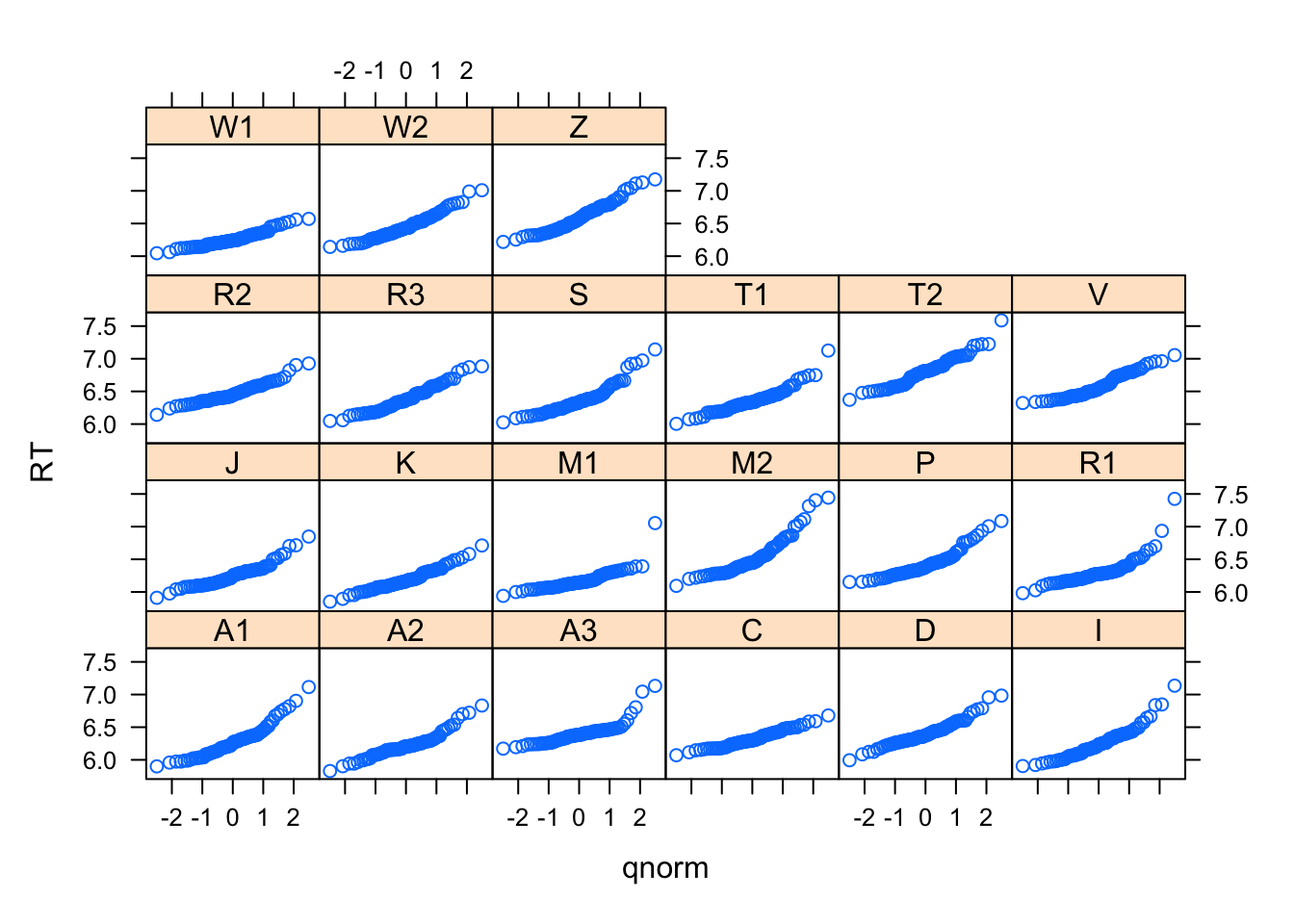
# across items
# qqmath(~RT|word, data = lexdec, layout = c(5,5,4))
3.4 Remove outlines
Here I will use densityplot to identify outlines but you can apply another principle e.g., +/- 3SD or criterium that is theoretically justified.
densityplot(lexdec$RT)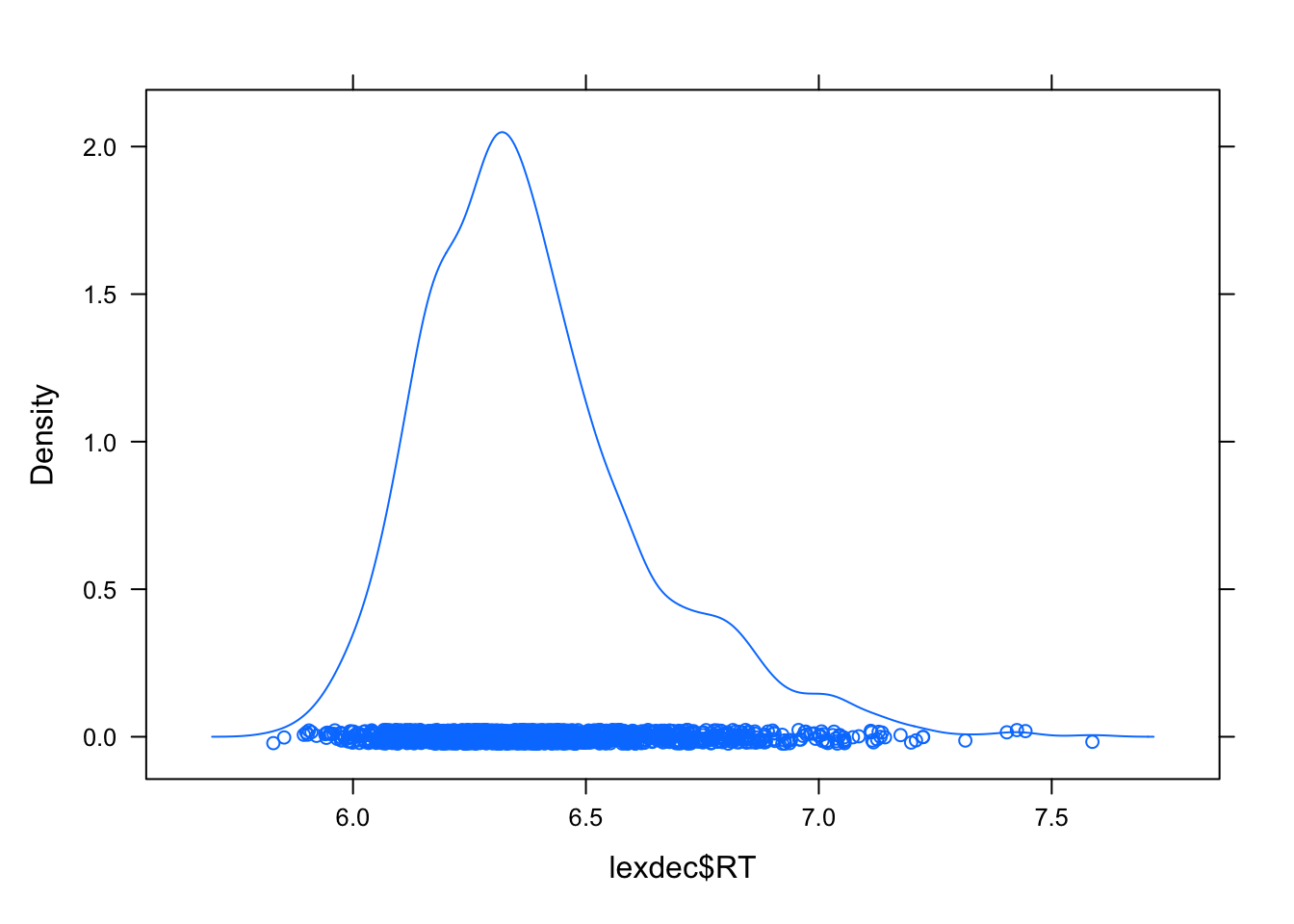
lexdec2 <- lexdec[lexdec$RT < 7 ,]
densityplot(lexdec2$RT)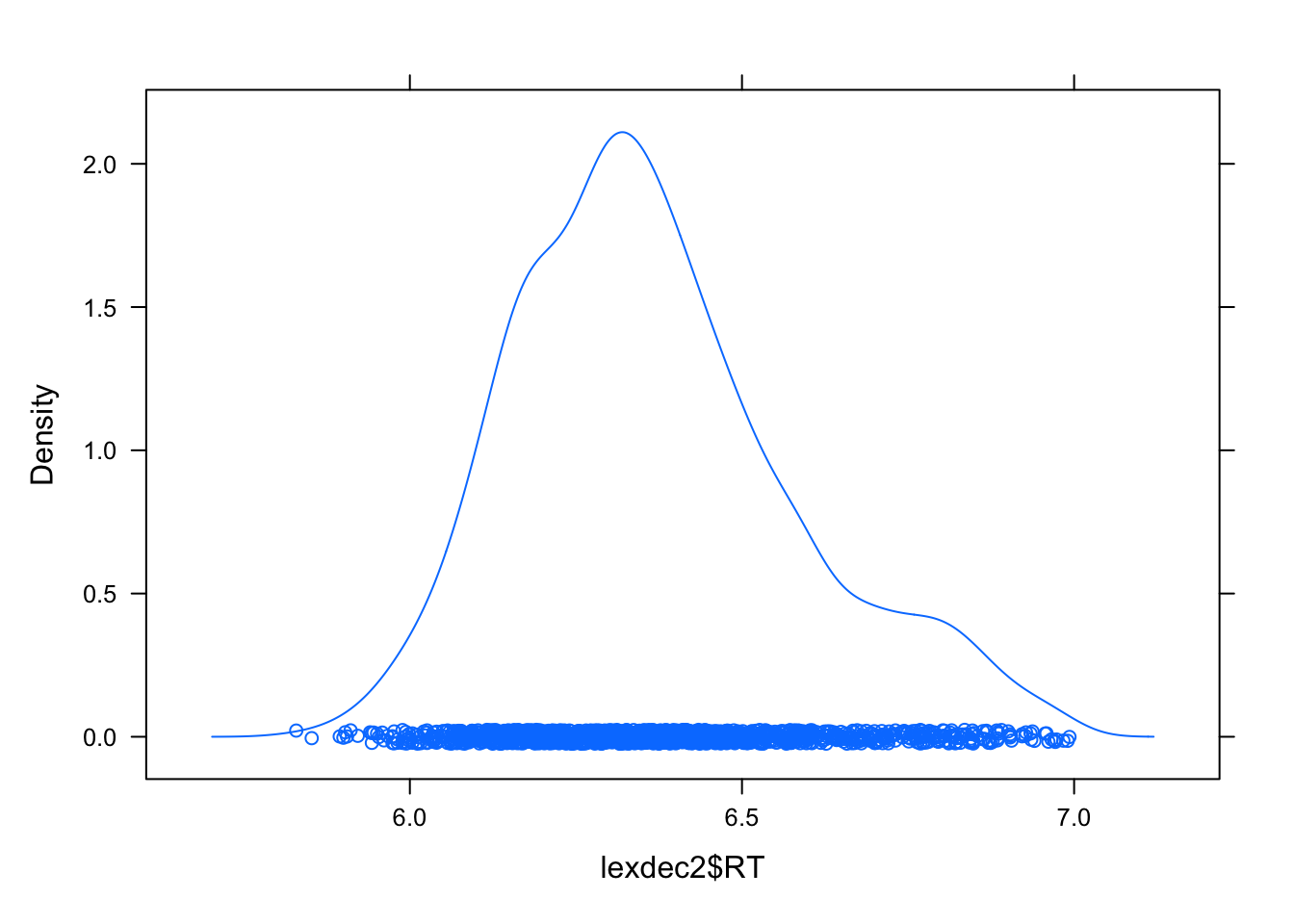
3.5 Identify fixed and random effects
Make sure that fixed and random effects are defined as factors and that your DV is in the appropriate class.
lexdec2$Subject<- as.factor(lexdec2$Subject)
lexdec2$Word <- as.factor(lexdec2$Word)
lexdec2$NativeLanguage <- as.factor(lexdec2$NativeLanguage)
lexdec2$RT <- as.numeric(lexdec2$RT)
str(lexdec2)
## 'data.frame': 1618 obs. of 28 variables:
## $ Subject : Factor w/ 21 levels "A1","A2","A3",..: 1 1 1 1 1 1 1 1 1 1 ...
## $ RT : num 6.34 6.31 6.35 6.19 6.03 ...
## $ Trial : int 23 27 29 30 32 33 34 38 41 42 ...
## $ Sex : Factor w/ 2 levels "F","M": 1 1 1 1 1 1 1 1 1 1 ...
## $ NativeLanguage: Factor w/ 2 levels "English","Other": 1 1 1 1 1 1 1 1 1 1 ...
## $ Correct : Factor w/ 2 levels "correct","incorrect": 1 1 1 1 1 1 1 1 1 1 ...
## $ PrevType : Factor w/ 2 levels "nonword","word": 2 1 1 2 1 2 2 1 1 2 ...
## $ PrevCorrect : Factor w/ 2 levels "correct","incorrect": 1 1 1 1 1 1 1 1 1 1 ...
## $ Word : Factor w/ 79 levels "almond","ant",..: 55 47 20 58 25 12 71 69 62 1 ...
## $ Frequency : num 4.86 4.61 5 4.73 7.67 ...
## $ FamilySize : num 1.386 1.099 0.693 0 3.135 ...
## $ SynsetCount : num 0.693 1.946 1.609 1.099 2.079 ...
## $ Length : int 3 4 6 4 3 10 10 8 6 6 ...
## $ Class : Factor w/ 2 levels "animal","plant": 1 1 2 2 1 2 2 1 2 2 ...
## $ FreqSingular : int 54 69 83 44 1233 26 50 63 11 24 ...
## $ FreqPlural : int 74 30 49 68 828 31 65 47 9 42 ...
## $ DerivEntropy : num 0.791 0.697 0.475 0 1.213 ...
## $ Complex : Factor w/ 2 levels "complex","simplex": 2 2 2 2 2 1 1 2 2 2 ...
## $ rInfl : num -0.31 0.815 0.519 -0.427 0.398 ...
## $ meanRT : num 6.36 6.42 6.34 6.34 6.3 ...
## $ SubjFreq : num 3.12 2.4 3.88 4.52 6.04 3.28 5.04 2.8 3.12 3.72 ...
## $ meanSize : num 3.48 3 1.63 1.99 4.64 ...
## $ meanWeight : num 3.18 2.61 1.21 1.61 4.52 ...
## $ BNCw : num 12.06 5.74 5.72 2.05 74.84 ...
## $ BNCc : num 0 4.06 3.25 1.46 50.86 ...
## $ BNCd : num 6.18 2.85 12.59 7.36 241.56 ...
## $ BNCcRatio : num 0 0.708 0.568 0.713 0.68 ...
## $ BNCdRatio : num 0.512 0.497 2.202 3.591 3.228 ...3.6 Center continuous predictors
Centering means subtracting the score from the grand mean. By centering the DV, we are moving its zero point to the center of the scale. As an effect, the intercept becomes interpretable. Centering has no effect on the relationship between the predictors and the outcome (i.e., coefficients will not change). However, fewer parameters are needed for model identification (i.e., faster computation).
lexdec2$c.Length <- lexdec2$Length - mean(lexdec2$Length) 3.7 Choose appropriate contrasts
Here, I want to examine to what extent the participant's native language influences the RT. I could hypothesis that non-native speakers are slower than native speakers and apply Treatment contrast.
lexdec2$NativeLanguage <- factor(lexdec2$NativeLanguage,
                            levels = c("English","Other"))
contrasts(lexdec2$NativeLanguage)
## Other
## English 0
## Other 13.8 Define the random structure
We have two fixed factors and two random factors Subject and Item. It is recommended to keep a maximal random effects structure (Barr et al., 2013). However, running a full random structure is challenging for at least three reasons:
- Processor time by adding additional parameters you significantly extend the computation time.
- Overparameterization which would increase the likelihood of Type II error.
- Failure to converge.
How to specify the random structure?
The rule of thumb is to start with removing correlations between fixed factors, then interactions, then random structure. First, trim down items then subjects.
Let's consider our example where we have two fixed factors (Native Language and Word Length) and two random factors (Subject and Word).
| model | random structure | |
|---|---|---|
| 1 | Full random structure | (1 + c.Length | Subject) + (1 + Native Language | Word) |
| 2 | Remove correlation from item | (1 + c.Length | Subject) + (0 + Native Language | Word) |
| 3 | Zero-covariances for item | (1 + c.Length | Subject) + (Native Language || Word) |
| 4 | Random intercept only for item | (1 + c.Length | Subject) + (1 | Word) |
| 5 | Remove correlation from subject | (0 + c.Length | Subject) + (1 | Word) |
| 6 | Zero-covariances for subject | (c.Length || Subject) + (Native Language || Word) |
| 7 | Random intercepts only model | (1 | Subject) + (1 | Word) |
# 1. Full random structure
lmer_1 <-lmer(RT ~ NativeLanguage*c.Length +
                    (1+c.Length| Subject) +(1+NativeLanguage| Word),
                  lexdec2)
## Warning in checkConv(attr(opt, "derivs"), opt$par, ctrl = control$checkConv, :
## Model failed to converge with max|grad| = 0.0025328 (tol = 0.002, component 1)
summary(lmer_1)


# 2. Remove correlation from item
lmer_2 <-lmer(RT ~ NativeLanguage*c.Length +
                    (1+c.Length| Subject) +(0+NativeLanguage| Word),
                  lexdec2)
summary(lmer_2)

# 3. Zero-covariances for item
lmer_3 <-lmer(RT ~ NativeLanguage*c.Length +
                    (1+c.Length| Subject) +(NativeLanguage || Word),
                  lexdec2)
## Warning in checkConv(attr(opt, "derivs"), opt$par, ctrl = control$checkConv, :
## unable to evaluate scaled gradient## Warning in checkConv(attr(opt, "derivs"), opt$par, ctrl = control$checkConv, :
## Model failed to converge: degenerate Hessian with 1 negative eigenvalues
summary(lmer_3)

# 4. Random intercepts only for item
lmer_4 <-lmer(RT ~ NativeLanguage*c.Length +
                    (1+c.Length| Subject) +(1| Word),
                  lexdec2)
summary(lmer_4)

# 5. Remove correlation from subject
lmer_5 <-lmer(RT ~ NativeLanguage*c.Length +
                    (0+ c.Length| Subject) +(1| Word),
                  lexdec2)
summary(lmer_5)

# 6. Zero-covariances for subject
lmer_6 <-lmer(RT ~ NativeLanguage*c.Length +
                    (c.Length || Subject) +(1| Word),
                  lexdec2)
summary(lmer_6)

# 7. Random intercepts only model
lmer_7 <-lmer(RT ~ NativeLanguage*c.Length +
                    (1| Subject) +(1| Word),
                  lexdec2)
summary(lmer_7)
## Linear mixed model fit by REML ['lmerMod']
## Formula: RT ~ NativeLanguage * c.Length + (1 + c.Length | Subject) + (1 +
## NativeLanguage | Word)
## Data: lexdec2
##
## REML criterion at convergence: -1308.8
##
## Scaled residuals:
## Min 1Q Median 3Q Max
## -2.4094 -0.6400 -0.0946 0.5129 4.2826
##
## Random effects:
## Groups Name Variance Std.Dev. Corr
## Word (Intercept) 0.002651 0.05149
## NativeLanguageOther 0.000401 0.02002 0.74
## Subject (Intercept) 0.016371 0.12795
## c.Length 0.000173 0.01315 0.73
## Residual 0.022568 0.15023
## Number of obs: 1618, groups: Word, 79; Subject, 21
##
## Fixed effects:
## Estimate Std. Error t value
## (Intercept) 6.312970 0.037707 167.423
## NativeLanguageOther 0.138994 0.056974 2.440
## c.Length 0.011378 0.005578 2.040
## NativeLanguageOther:c.Length 0.015238 0.007195 2.118
##
## Correlation of Fixed Effects:
## (Intr) NtvLnO c.Lngt
## NtvLnggOthr -0.642
## c.Length 0.484 -0.321
## NtvLnggO:.L -0.376 0.581 -0.463
## optimizer (nloptwrap) convergence code: 0 (OK)
## Model failed to converge with max|grad| = 0.0025328 (tol = 0.002, component 1)
##
## Linear mixed model fit by REML ['lmerMod']
## Formula: RT ~ NativeLanguage * c.Length + (1 + c.Length | Subject) + (0 +
## NativeLanguage | Word)
## Data: lexdec2
##
## REML criterion at convergence: -1308.8
##
## Scaled residuals:
## Min 1Q Median 3Q Max
## -2.4095 -0.6401 -0.0946 0.5130 4.2826
##
## Random effects:
## Groups Name Variance Std.Dev. Corr
## Word NativeLanguageEnglish 0.0026501 0.05148
## NativeLanguageOther 0.0045758 0.06764 0.98
## Subject (Intercept) 0.0163712 0.12795
## c.Length 0.0001729 0.01315 0.73
## Residual 0.0225680 0.15023
## Number of obs: 1618, groups: Word, 79; Subject, 21
##
## Fixed effects:
## Estimate Std. Error t value
## (Intercept) 6.312970 0.037706 167.424
## NativeLanguageOther 0.138994 0.056974 2.440
## c.Length 0.011378 0.005577 2.040
## NativeLanguageOther:c.Length 0.015238 0.007193 2.118
##
## Correlation of Fixed Effects:
## (Intr) NtvLnO c.Lngt
## NtvLnggOthr -0.642
## c.Length 0.484 -0.321
## NtvLnggO:.L -0.376 0.581 -0.463
## Linear mixed model fit by REML ['lmerMod']
## Formula: RT ~ NativeLanguage * c.Length + (1 + c.Length | Subject) + ((1 |
## Word) + (0 + NativeLanguage | Word))
## Data: lexdec2
##
## REML criterion at convergence: -1308.8
##
## Scaled residuals:
## Min 1Q Median 3Q Max
## -2.4095 -0.6401 -0.0946 0.5130 4.2827
##
## Random effects:
## Groups Name Variance Std.Dev. Corr
## Word NativeLanguageEnglish 0.0015002 0.03873
## NativeLanguageOther 0.0034257 0.05853 1.00
## Word.1 (Intercept) 0.0011501 0.03391
## Subject (Intercept) 0.0163714 0.12795
## c.Length 0.0001729 0.01315 0.73
## Residual 0.0225680 0.15023
## Number of obs: 1618, groups: Word, 79; Subject, 21
##
## Fixed effects:
## Estimate Std. Error t value
## (Intercept) 6.312970 0.037707 167.423
## NativeLanguageOther 0.138994 0.056974 2.440
## c.Length 0.011378 0.005577 2.040
## NativeLanguageOther:c.Length 0.015238 0.007194 2.118
##
## Correlation of Fixed Effects:
## (Intr) NtvLnO c.Lngt
## NtvLnggOthr -0.642
## c.Length 0.484 -0.321
## NtvLnggO:.L -0.376 0.581 -0.463
## optimizer (nloptwrap) convergence code: 0 (OK)
## unable to evaluate scaled gradient
## Model failed to converge: degenerate Hessian with 1 negative eigenvalues
##
## Linear mixed model fit by REML ['lmerMod']
## Formula: RT ~ NativeLanguage * c.Length + (1 + c.Length | Subject) + (1 |
## Word)
## Data: lexdec2
##
## REML criterion at convergence: -1305.6
##
## Scaled residuals:
## Min 1Q Median 3Q Max
## -2.3539 -0.6550 -0.0918 0.5069 4.2598
##
## Random effects:
## Groups Name Variance Std.Dev. Corr
## Word (Intercept) 0.0033226 0.05764
## Subject (Intercept) 0.0163091 0.12771
## c.Length 0.0001724 0.01313 0.73
## Residual 0.0226760 0.15059
## Number of obs: 1618, groups: Word, 79; Subject, 21
##
## Fixed effects:
## Estimate Std. Error t value
## (Intercept) 6.312985 0.037752 167.221
## NativeLanguageOther 0.138511 0.056825 2.437
## c.Length 0.011383 0.005794 1.965
## NativeLanguageOther:c.Length 0.015203 0.007089 2.144
##
## Correlation of Fixed Effects:
## (Intr) NtvLnO c.Lngt
## NtvLnggOthr -0.645
## c.Length 0.463 -0.308
## NtvLnggO:.L -0.379 0.589 -0.520
## Linear mixed model fit by REML ['lmerMod']
## Formula: RT ~ NativeLanguage * c.Length + (0 + c.Length | Subject) + (1 |
## Word)
## Data: lexdec2
##
## REML criterion at convergence: -608.1
##
## Scaled residuals:
## Min 1Q Median 3Q Max
## -2.9126 -0.6881 -0.0985 0.5731 3.5047
##
## Random effects:
## Groups Name Variance Std.Dev.
## Word (Intercept) 0.0021929 0.04683
## Subject c.Length 0.0001046 0.01023
## Residual 0.0377561 0.19431
## Number of obs: 1618, groups: Word, 79; Subject, 21
##
## Fixed effects:
## Estimate Std. Error t value
## (Intercept) 6.312913 0.008237 766.389
## NativeLanguageOther 0.129495 0.009801 13.213
## c.Length 0.011420 0.005331 2.142
## NativeLanguageOther:c.Length 0.012081 0.006939 1.741
##
## Correlation of Fixed Effects:
## (Intr) NtvLnO c.Lngt
## NtvLnggOthr -0.496
## c.Length -0.007 0.003
## NtvLnggO:.L 0.002 0.003 -0.551
## Linear mixed model fit by REML ['lmerMod']
## Formula: RT ~ NativeLanguage * c.Length + ((1 | Subject) + (0 + c.Length |
## Subject)) + (1 | Word)
## Data: lexdec2
##
## REML criterion at convergence: -1297.6
##
## Scaled residuals:
## Min 1Q Median 3Q Max
## -2.3904 -0.6517 -0.0909 0.5031 4.2687
##
## Random effects:
## Groups Name Variance Std.Dev.
## Word (Intercept) 0.0033153 0.05758
## Subject c.Length 0.0001695 0.01302
## Subject.1 (Intercept) 0.0162536 0.12749
## Residual 0.0226801 0.15060
## Number of obs: 1618, groups: Word, 79; Subject, 21
##
## Fixed effects:
## Estimate Std. Error t value
## (Intercept) 6.31297 0.03769 167.498
## NativeLanguageOther 0.13823 0.05673 2.437
## c.Length 0.01137 0.00577 1.970
## NativeLanguageOther:c.Length 0.01499 0.00705 2.126
##
## Correlation of Fixed Effects:
## (Intr) NtvLnO c.Lngt
## NtvLnggOthr -0.645
## c.Length -0.001 0.000
## NtvLnggO:.L 0.000 0.000 -0.519
## Linear mixed model fit by REML ['lmerMod']
## Formula: RT ~ NativeLanguage * c.Length + (1 | Subject) + (1 | Word)
## Data: lexdec2
##
## REML criterion at convergence: -1281.3
##
## Scaled residuals:
## Min 1Q Median 3Q Max
## -2.9909 -0.6566 -0.1023 0.5245 4.3696
##
## Random effects:
## Groups Name Variance Std.Dev.
## Word (Intercept) 0.003287 0.05734
## Subject (Intercept) 0.016181 0.12720
## Residual 0.023243 0.15246
## Number of obs: 1618, groups: Word, 79; Subject, 21
##
## Fixed effects:
## Estimate Std. Error t value
## (Intercept) 6.313047 0.037612 167.845
## NativeLanguageOther 0.137691 0.056618 2.432
## c.Length 0.011387 0.004386 2.596
## NativeLanguageOther:c.Length 0.014458 0.004137 3.495
##
## Correlation of Fixed Effects:
## (Intr) NtvLnO c.Lngt
## NtvLnggOthr -0.645
## c.Length -0.002 0.000
## NtvLnggO:.L 0.001 0.001 -0.395Let's now compare models 4, 5, 6, and 7.
anova(lmer_5, lmer_4)| npar | AIC | BIC | logLik | deviance | Chisq | Df | Pr(>Chisq) | |
|---|---|---|---|---|---|---|---|---|
| lmer_5 | 7 | -626.7357 | -589.0131 | 320.3679 | -640.7357 | NA | NA | NA |
| lmer_4 | 9 | -1314.3479 | -1265.8474 | 666.1739 | -1332.3479 | 691.6122 | 2 | 0 |
The AIC and BIC are criteria for model selection that measures the trade-off between model fit and complexity of the model. A lower AIC or BIC value indicates a better fit.
3.10 Task 1
Let's warm up!
Using lexdec data file test to what extent RT is predicted by word complexity (i.e., Complex) and whether this effect is modulated by the position of a trial in the experiment (i.e., Trial). Apply Treatment contrast to test hypothesis that simpler words are process faster than complex one.
lexdec2$c.Trial <- lexdec2$Trial - mean(lexdec2$Trial)

lexdec2$Complex<- factor(lexdec2$Complex,
                            levels = c("simplex", "complex"))
contrasts(lexdec2$Complex)


# 1. Full random structure
lmer_task1 <-lmer(RT ~ Complex*c.Trial +
                    (1+Complex| Subject) +(1| Word),
                  lexdec2)
summary(lmer_task1)
## complex
## simplex 0
## complex 1
## Linear mixed model fit by REML ['lmerMod']
## Formula: RT ~ Complex * c.Trial + (1 + Complex | Subject) + (1 | Word)
## Data: lexdec2
##
## REML criterion at convergence: -1247.8
##
## Scaled residuals:
## Min 1Q Median 3Q Max
## -2.4238 -0.6555 -0.0993 0.5371 4.4071
##
## Random effects:
## Groups Name Variance Std.Dev. Corr
## Word (Intercept) 0.004325 0.06577
## Subject (Intercept) 0.018981 0.13777
## Complexcomplex 0.002103 0.04586 0.78
## Residual 0.023131 0.15209
## Number of obs: 1618, groups: Word, 79; Subject, 21
##
## Fixed effects:
## Estimate Std. Error t value
## (Intercept) 6.369e+00 3.135e-02 203.157
## Complexcomplex 2.503e-02 2.699e-02 0.928
## c.Trial -2.083e-04 8.752e-05 -2.381
## Complexcomplex:c.Trial -3.038e-05 2.477e-04 -0.123
##
## Correlation of Fixed Effects:
## (Intr) Cmplxc c.Tril
## Complxcmplx 0.184
## c.Trial 0.001 -0.002
## Cmplxcmp:.T 0.000 -0.028 -0.3563.11 Homework
Using lexdec data file test to what extent RT is predicted by the interaction between word length and participants' native language. In your model control for the effect of trial and word frequency (i.e., Frequency). Consider correct responses only. Conduct intercept only model.
lexdec2$c.Frequency <- lexdec2$Frequency - mean(lexdec2$Frequency)

# 1. Full random structure
lmer_task2 <-lmer(RT ~ NativeLanguage*c.Length + c.Trial + c.Frequency +
                    (1| Subject) +(1| Word),
                  lexdec2[lexdec2$Correct ==
"correct",]) # correct responses only
summary(lmer_task2)
## Linear mixed model fit by REML ['lmerMod']
## Formula: RT ~ NativeLanguage * c.Length + c.Trial + c.Frequency + (1 |
## Subject) + (1 | Word)
## Data: lexdec2[lexdec2$Correct == "correct", ]
##
## REML criterion at convergence: -1290.1
##
## Scaled residuals:
## Min 1Q Median 3Q Max
## -2.2840 -0.6679 -0.1121 0.5215 4.4047
##
## Random effects:
## Groups Name Variance Std.Dev.
## Word (Intercept) 0.00213 0.04615
## Subject (Intercept) 0.01482 0.12175
## Residual 0.02231 0.14937
## Number of obs: 1557, groups: Word, 79; Subject, 21
##
## Fixed effects:
## Estimate Std. Error t value
## (Intercept) 6.316e+00 3.587e-02 176.087
## NativeLanguageOther 1.359e-01 5.424e-02 2.506
## c.Length 2.444e-03 4.199e-03 0.582
## c.Trial -1.938e-04 8.127e-05 -2.384
## c.Frequency -3.226e-02 5.607e-03 -5.753
## NativeLanguageOther:c.Length 1.698e-02 4.156e-03 4.087
##
## Correlation of Fixed Effects:
## (Intr) NtvLnO c.Lngt c.Tril c.Frqn
## NtvLnggOthr -0.647
## c.Length -0.001 0.000
## c.Trial -0.001 0.001 0.009
## c.Frequency 0.001 -0.002 0.391 0.005
## NtvLnggO:.L 0.001 0.004 -0.408 -0.029 -0.002